The Grimoire: Tome of Cursed Knowledge

This is the place where I collect all the knowledge earned during my self taught computer science journey, a grimoire that freely, available to be consulted at any time.

Rather than leaving my notes scattered across random bookmarks, Discord servers, notebooks and Google Docs, this grimoire serves as a single source of truth for all the things that I'm learning during in this tedious, painful path.

If you're reading this, you're either past-me, future-me, or an unfortunate soul who has stumbled upon my secret knowledge. Either way, remember:

🛠️ Debugging is an art, not a science.
💀 Despite accumulating knowledge, there will still always be a moment where you'll be thrown into the unknown, left to figure it out. That's just how things are.

Setting Up SSH for GitHub

This will make GitHub stop asking you for your username and access token every time.

Step 1: Check if you already have a key

Before generating a new one, check if you already have an SSH key:

ls -al ~/.ssh

If you see files like id_rsa and id_rsa.pub (or id_ed25519 and id_ed25519.pub), you probably already have an SSH key. If not, generate one.

Step 2: Generate a New SSH key (if needed)

If you don't have an existing SSH key, generate a new one:

ssh-keygen -t ed25519 -C "yourmail@example.com"

When it asks for a file location, just press Enter (this will save it in ~/.ssh/id_ed25519).
When it asks for a passphrase, you can leave it empty (or set one for extra security).

Step 3: Add Your SSH Key to the SSH Agent

Now, you need to add the key to your local SSH agent so it gets used automatically:

eval "$(ssh-agent -s)"

Then add your key:

ssh-add ~/.ssh/id_ed25519

(If you used rsa, replace id_ed25519 with id_rsa.)

Step 4: Copy Your SSH Key to GitHub

Now, you need to add your SSH key to your GitHub account.

Copy the key to your clipboard:

cat ~/.ssh/id_ed25519.pub

It will output something like:

ssh-ed25519 AAAAC3Nza...yourlongpublickeyhere yourmail@example.com

Go to GitHub → SSH Keys Settings
Click "New SSH Key", paste your key, and give it a name.
Save it.

Step 5: Test the Connection

Check if GitHub recognizes your SSH key:

ssh -T git@github.com

If everything is set up correctly, you should see:

Hi <your-github-username>! You've successfully authenticated, but GitHub does not provide shell access.

Step 6: Change Your Git Remote to Use SSH

If your Git remote is still using HTTPS (which asks for a password), switch it to SSH:

git remote -v

If you see:

origin https://github.com/your-username/repository.git (fetch)
origin https://github.com/your-username/repository.git (push)

Change it to SSH:

git remote set-url origin git@github.com:your-username/repository.git

Now, every push/pull will use SSH, and you’ll never have to enter your password again.

The Skinny Ruby Queen: Minimal Dockerfile for Production

1. Build Stage

We're building in style. Ruby + Alpine = skinny legend

FROM ruby:3.3-alpine AS build

Install a full dev toolchain to compile native gems (yes, Ruby still lives in C land)

RUN apk add --no-cache build-base

Set the working directory—aka the sacred ground where it all happens

WORKDIR /usr/src/app

Copy only Gemfile and lockfile first (layer caching magic)

COPY Gemfile Gemfile.lock ./

Configure bundler to install gems locally under vendor/bundle. This will be copied over to the final image later like a blessed artifact

RUN bundle config set --local path 'vendor/bundle' \
  && bundle install

Copy the rest of your application—code, chaos, and all

COPY . .

2. Final Stage

A clean Alpine base with Ruby and none of that build baggage. We like our containers light.

FROM ruby:3.3-alpine

Set the working dir again (yes, you need to re-declare it—Docker has no memory of its past life)

WORKDIR /usr/src/app

Copy everything from the build stage, including those precious compiled gems

COPY --from=build /usr/src/app /usr/src/app

Let Ruby know where the gems are—because it forgets if you don’t tell it

ENV GEM_PATH=/usr/src/app/vendor/bundle/ruby/3.3.0
ENV PATH=$GEM_PATH/bin:$PATH

Install only the runtime dependencies needed for your app to vibe

RUN apk add --no-cache \
        libstdc++ \       # C++ runtime
        libffi \          # Needed by some gems (e.g., FFI, psych)
        yaml \            # YAML parsing
        zlib \            # Compression stuff
        openssl \         # HTTPS, TLS, etc.
        tzdata            # So your logs don’t think it's 1970

Declare yourself: prod mode on

ENV RACK_ENV=production
ENV PORT=8080
EXPOSE 8080

Finally, launch the Ruby app like the main character it is

CMD ["ruby", "server.rb"]

Some useful commands:

docker build -t your-image-name .

docker images

docker run -p 8080:8080 your-image-id

docker rmi your-image-id

docker container prune

Pro Tips from the Underworld: If you're using gems that compile C extensions (like pg, nokogiri, ffi), you’ll likely need additional Alpine dependencies, e.g.:

RUN apk add --no-cache build-base libxml2-dev libxslt-dev postgresql-dev

For scripts that are long-running, consider using:

CMD ["ruby", "start.rb"]

Or even:

CMD ["rackup", "--host", "0.0.0.0", "--port", "8080"]

Deploying mdBook to GitHub Pages With GitHub Actions

Step 1: Setup the Repo

Create a new GitHub repo.
Run:

cargo install mdbook
mdbook init my-docs
cd my-docs

Step 2: Add GitHub Actions Workflow

Create .github/workflows/deploy.yml:

name: Deploy mdBook to GitHub Pages

on:
  push:
    branches:
      - main

jobs:
  deploy:
    runs-on: ubuntu-latest

    steps:
      - name: Checkout repository
        uses: actions/checkout@v3

      - name: Install mdBook
        run: cargo install mdbook

      - name: Build the book
        run: mdbook build

      - name: Setup SSH Authentication
        run: |
          mkdir -p ~/.ssh
          echo "${{ secrets.SSH_PRIVATE_KEY }}" > ~/.ssh/id_ed25519
          chmod 600 ~/.ssh/id_ed25519
          ssh-keyscan github.com >> ~/.ssh/known_hosts

      - name: Deploy to GitHub Pages
        uses: peaceiris/actions-gh-pages@v3
        with:
          github_token: ${{ secrets.GITHUB_TOKEN }}
          publish_dir: ./book

SSH_PRIVATE_KEY -> (id_ed25519) GITHUB_TOKEN -> GitHub adds this automatically

Step 3: Add Secrets

Generate a separate SSH key for CI/CD

ssh-keygen -t ed25519 -C "GitHub Actions Deploy Key"

Go to Repo -> Settings -> Secrets and Variables -> Actions
Add SSH_PRIVATE_KEY -> Paste the private key (id_ed25519)
Go to Repo -> Settings -> Deploy key
Paste the public key (id_ed25519.pub)

Step 4: Enable Permissions

Go to Repo -> Settings -> Actions -> General
Under Workflow Permissions, enable: ✅ Read and Write Permissions ✅ Allow GitHub Actions to create and approve pull requests

Step 5: Push and Deploy

git add .
git commit -m "Deploy Book"
git push origin main

If it all goes well, your docs should be live.

CI/CD Pipeline Setup for Cloud Run

Deploy your projects automatically with a simple git commit and git push. To do this, you need to Install the gcloud CLI

Step 1: Test Locally with Docker

Build the image and test before pushing anything to Google Cloud.

docker build -t my-portfolio .
docker run -p 8080:8080 my-portfolio

Fix any port, environment, or dependency issues locally first.
Once it works locally, move on to Google Cloud.

Step 2: Set Up Google Cloud

Before running these commands, be sure to:
- Check current GCP project:
```
gcloud config list project
```
- Set active project
```
gcloud config set project YOUR_PROJECT_ID
```
- You can also view all projects your account can access:
```
gcloud projects list
```
Enable the required APIs (run these in your terminal):

gcloud services enable \
  cloudbuild.googleapis.com \
  run.googleapis.com \
  artifactregistry.googleapis.com

This ensures Google Cloud has all necessary services activated.

Create an Artifact Registry repo for Docker images:

gcloud artifacts repositories create portfolio-repo \
  --repository-format=docker \
  --location=europe-west1 \
  --description="Docker repository for portfolio deployment"

This stores your container images so Cloud Run can pull them.

Step 3: Create a Service Account for GitHub Actions

Create a user for CI/CD:

gcloud iam service-accounts create github-deployer \
  --description="GitHub Actions service account" \
  --display-name="GitHub Deployer"

This creates a dedicated user for deploying the app.

Grant it permissions:

gcloud projects add-iam-policy-binding $YOUR_PROJECT_ID \
  --member=serviceAccount:github-deployer@$YOUR_PROJECT_ID.iam.gserviceaccount.com \
  --role=roles/run.admin

gcloud projects add-iam-policy-binding $YOUR_PROJECT_ID \
  --member=serviceAccount:github-deployer@$YOUR_PROJECT_ID.iam.gserviceaccount.com \
  --role=roles/artifactregistry.writer

gcloud projects add-iam-policy-binding $YOUR_PROJECT_ID \
  --member=serviceAccount:github-deployer@$YOUR_PROJECT_ID.iam.gserviceaccount.com \
  --role=roles/storage.admin

GitHub Actions can now push images & deploy to Cloud Run.

Generate a key file for the service account:

gcloud iam service-accounts keys create key.json \
  --iam-account=github-deployer@$YOUR_PROJECT_ID.iam.gserviceaccount.com

This creates key.json, which contains the credentials.

Add Secrets to GitHub

Go to your GitHub repo -> Settings -> Secrets and Variables -> Actions
Add two secrets in Secrets -> repository secrets:

1.GCP_SERVICE_ACCOUNT_KEY → Copy & paste the full contents of key.json.

2.GCP_PROJECT_ID → Your Google Cloud project ID.

Now, GitHub Actions can authenticate with Google Cloud

Step 5: Create GitHub Actions Workflows (`deploy.yml`)

In your repo, create: .github/workflows/deploy.yml

name: Deploy to Cloud Run

on:
  push:
    branches:
      - main

jobs:
  deploy:
    runs-on: ubuntu-latest

    steps:
      - name: Checkout repository
        uses: actions/checkout@v3

      - name: Authenticate with Google Cloud
        uses: google-github-actions/auth@v2
        with:
          credentials_json: ${{ secrets.GCP_SERVICE_ACCOUNT_KEY }}
      
      - name: Set Up Google Cloud SDK
        run: |
          gcloud auth configure-docker europe-west2-docker.pkg.dev

      - name: Build and push Docker Image
        run: |
          docker build -t europe-west1-docker.pkg.dev/${{ secrets.GCP_PROJECT_ID }}/portfolio-repo/portfolio .
          docker push europe-west1-docker.pkg.dev/${{ secrets.GCP_PROJECT_ID }}/portfolio-repo/portfolio

      - name: Deploy to Cloud Run
        run: |
          gcloud run deploy portfolio-site \
          --image europe-west1-docker.pkg.dev/${{ secrets.GCP_PROJECT_ID }}/portfolio-repo/portfolio \
          --platform managed \
          --region europe-west1 \
          --allow-unauthenticated

Now, every push to main will automatically deploy to Cloud Run.

Step 6: Push & Deploy

Once everything is set up:

git add .
git commit -m "Setup GitHub Actions CI/CD"
git push origin main

Check GitHub Actions -> It should build & deploy your project automatically.

Adding a Domain to Google Cloud Run

I have unfortunately decided to swallow my pride and use the Google Cloud UI for this one.

Step 1: Set Up Domain Mapping

Go to the google cloud console -> select the Cloud Run service.
Click "Manage custom domains"
CLick Add Mapping -> "Add service domain mapping"
Select the service you want to map to -> select your deployed project.
Enter your domain name -> Click "Continue"
Google Cloud will generate DNS records -> copy these

Step 2: Update DNS Settings in Your Domain Host**

Go to your domain provider (Cloudflare, Namecheap, Google Domains, etc.).
Paste the DNS records exactly as given.
If you are using Cloudflare, set your records to "DNS Only" (disabling proxy mode) so Google can verify them.

Step 3: Verify the DNS Changes

While waiting, feel free to test your domain name on nslookup.io.
If the IPv4 and IPv6 addresses matches what Google gave you, then you're good.

Bonus: Enable Subdomains

Bonus: in your domain host DNS settings, add * as a host, CNAME as type and ghs.googlehosted.com if you want subdomains.

-Now any subdomain (blog.yourdomain.com, api.yourdomain.com, etc.) will automatically work.

Fix: If Your Cloud Run Region Doesn’t Support Domain Mapping

🔥 If you see:

❌ "Domain mappings are not available in this region."

💀 Google Cloud decided your region isn’t good enough.

Just edit the YAML file in your repository to switch to a supported one.
Commit and push the change.
In your Cloud Run services, remove the old container.

How to configure Google Cloud Storage Bucket to store any files

Create a Google Cloud Storage Bucket. Make sure to pick a unique bucket name!
Example locations: us-central1, europe-west2, asia-east1.

gcloud storage buckets create gs://UNIQUE_BUCKET_NAME
--location=SERVER_LOCATION
--uniform-bucket-level-access

# Navigate to your folder path
cd ~/Downloads

# Upload the entire "public" folder
gsutil cp -r /public gs://UNIQUE_BUCKET_NAME

# Upload a single file, or an entire folder (later updates)
gsutil cp myfile.png gs://UNIQUE_BUCKET_NAME
gsutil cp -r myfolder gs://UNIQUE_BUCKET_NAME

# Automate Upload with Wildcards (this uploads all .jpg files in the current directory)
gsutil cp *.jpg gs://UNIQUE_BUCKET_NAME

# (Optional) Make files Public. This will make the files publicly accessed via URL.
gsutil iam ch allUsers:objectViewer gs://UNIQUE_BUCKET_NAME

# Access to an image in the folder with your web browser, once uploaded.
https://storage.googleapis.com/UNIQUE_BUCKET_NAME/your-file.jpg

# List Files in the Bucket
gsutil ls gs://UNIQUE_BUCKET_NAME

# Delete Files (if needed)
gsutil rm gs://UNIQUE_BUCKET_NAME/filename.png

Set Up PostgreSQL in a Google Cloud VM using Docker Compose

1. Google Cloud Prep

Make sure you have a Google Cloud Project set up.
Enable Billing, Compute Engine, and Cloud SQL Admin API.
Create a VM instance (Debian, obviously).

2. Generate SSH key locally:

ssh-keygen -t rsa -b 4096 -C "pwatpwat@yourdomain.dev"

Hit Enter a few times to use default paths (~/.ssh/id_rsa).

3. Connect to the VM instance

Connect

gcloud config set project pwatgres

pwatgres = project name.

Check if the first connection worked:

gcloud config list

Add your SSH key to the project:

gcloud compute os-login ssh-keys add --key-file=~/.ssh/id_rsa.pub

Confirm access:

gcloud compute ssh pwat-db-vm --zone=europe-west1-b

Basic Post-Boot Hardening

Firewall with ufw:

sudo apt update && sudo apt upgrade -y
sudo apt install ufw -y
sudo ufw allow OpenSSH
sudo ufw enable

Fail2Ban (basic brute-force protection)

sudo apt install fail2ban -y
sudo systemctl enable fail2ban
sudo systemctl start fail2ban

4. Docker Setup

sudo apt update && sudo apt install docker.io -y
sudo systemctl enable docker
sudo systemctl start docker

Test if the daemon hears your call:

docker --version

Install Docker Compose:

sudo apt install docker-compose -y
docker-compose --version

Let Yourself Command the Docker Army

sudo usermod -aG docker $USER
newgrp docker

You now have Docker privileges without needing sudo every time like a mortal.

5. Create Docker Compose Project

mkdir ~/pwatgres && cd ~/pwatgres
nano docker-compose.yml

version: '3.8'
services:
  postgres:
    image: postgres:16
    restart: always
    container_name: pwatgres
    env_file:
      - .env
    ports:
      - "5432:5432"
    volumes:
      - pgdata:/var/lib/postgresql/data
volumes:
  pgdata:

Create the .env file

Inside ~/pwatgres/:

nano .env

Example contents:

POSTGRES_DB=mydb
POSTGRES_USER=admin
POSTGRES_PASSWORD=changemepls

Save and close. DO NOT commit this if you ever sync this repo.

You can lock this .env file down with:

chmod 600 .env

Deploy that beast

docker-compose up -d

Misc

To shut down gracefully:

sudo shutdown +1 "The API layer dreams tonight. Goodnight, sweet daemon."

Security: Avoid Paying for Google’s Mistakes

Set up a billing alert. If your database starts scaling up unnecessarily, you will get charged.
Limit instance size in Compute Engine (e.g., ec2-nano).

Create an HMAC Server API with Python

from fastapi import FastAPI, Request, HTTPException
import hmac
import hashlib

app = FastAPI()


def calc_digest(key, message):
    key = bytes(key, 'utf-8')
    message = bytes(message, 'utf-8')
    dig = hmac.new(key, message, hashlib.sha256)
    return dig.hexdigest()

# HMAC Server
@app.post("/verify")
async def verify_signature(request: Request):
    body = await request.json()
    recieved_mac = request.headers.get("X-HMAC-Signature")

    if not recieved_mac:
        raise HTTPException(status_code=400, detail="Missing HMAC header")

    msg_string = f"{body['mac_address']}:{body['timestamp']}"
    expected_mac = calc_digest('secret-key', msg_string)

    if not hmac.compare_digest(recieved_mac, expected_mac):
        raise HTTPException(status_code=403, detail="Invalid signature")

    return {"status": "Verified"}

Testing HMAC Protected Endpoints with curl (Bash Script)

#!/bin/bash

MESSAGE='{"mac_address":"12:34:56:78:9a:bc","timestamp":"2025-04-30T15:00:00"}'
SIGNATURE=$(echo -n '{"mac_address":"12:34:56:78:9a:bc","timestamp":"2025-04-30T15:00:00"}' |
  openssl dgst -sha256 -hmac "secret-key" | sed 's/^.* //')

curl -X POST http://127.0.0.1:8000/verify \
  -H "Content-Type: application/json" \
  -H "X-HMAC-Signature: $SIGNATURE" \
  -d "$MESSAGE"

Establish connection with an HMAC client (for example, with Ruby)

require 'openssl/hmac'
require 'mac-address'

# HMAC Client
class Hmac
  def self.call
    key = secret_key
    mac_address = MacAddress.address
    halt 404, 'Mac Address not found' if mac_address.nil?

    timestamp = Time.now.to_i
    message = "#{mac_address}:#{timestamp}"
    mac = calc_digest(key, message)
    { signature: mac, timestamp: timestamp, mac_address: mac_address }
  end

  def self.secret_key
    ENV['API_DB_KEY'] || raise('Missing API_DB_KEY')
  end

  def self.calc_digest(key, message)
    OpenSSL::HMAC.hexdigest('sha256', key, message)
  end
end

Set up a LAMP server

Prerequisites: Type 2 hypervisor. In this guide, we're going to use VirtualBox (but you can always use virt-manager on Linux).

Configuring a Debian VM:

Downloading Debian on www.debian.org (this will be the operating system on which will run the virtual machine.
Download, install and configure VirtualBox and VirtualBox Extension Pack
For VirtualBox: accept everything and proceed.

Debian

For VirtualBox Extensions Pack:

Open the downloaded file
Click on Installation
Accept the terms of service
Tools → Extensions hamburger menu to check that the extension is installed.

Creation of the Debian Virtual Machine:

Debian VM

Choose an appropriate name for the VM
Choose the Debian ISO image you downloaded earlier
Check "Skip Unattended Installation"

Debian VM 2

Resources to be assigned: 2048MB of RAM, 1-2 CPUs and 10-20GB of hard drive.
Click "Finish", and you should see the machine appear in the VM list if there are no problems.

Additional Configurations:

Enable shared clipboard and drag and drop in General → Advanced

Shared Clipboard

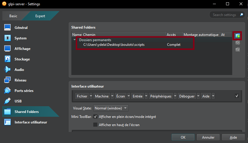
Enable shared folders in Settings → Shared Folders (here I added a scripts folder)

Shared Folders

In the "System" tab, change the boot order to:

Hard Drive (Checked)
Optical Drive (Checked)
Floppy Drive (Unchecked)
Network Drive (Unchecked)

Debian VM 3

In the "Display" tab → Screen, increase the "Video Memory" slider to 128MB and check the "Enable 3D Acceleration" box.
In the "Network" tab, check that the "Enable Network Interface" and "Cable Connected" boxes are enabled. The network access mode must also be set to "NAT".
In the "USB" tab, enable the USB controller and check the "USB 3.0 Controller (xHCI)" button.

You may finally boot up the Debian Virtual Machine.

Initialization

Partition formatting: Yes.
At the taskbar step, Debian will ask you to choose which software to pre-install. You must check "SSH Server," leave "Common System Utilities" checked, and check "XFCE Desktop", or a different one of your convenience.
Install the GRUB boot program: Yes, and select the disk that appears.

Guest Addons

VirtualBox Guest Additions:

In the menu bar, click "Devices", then "Insert Guest Additions CD Image".
Access the optical drive that just appeared.
Right-click → open a terminal.
Become root by running the su command and entering your password.
Enter the command sh ./VboxLinuxAdditions.run to start the installation of the "Guest Additions".
Restart the VM.
Make sure that in the "Devices" menu, "Shared Clipboard" and "Drag & Drop" are checked to "Bidirectional".
Right Ctrl + f: to enable/disable full screen.

GLPI Installation

Once Debian is installed, create a Bash script called setup_glpi.sh that will set up the LAMP stack. This script requires root access.
The LAMP stack consists of the Apache2 web server, a MariaDB database and the PHP language.
If "sudo" doesn't work for some reason, you can use "su" instead for the time being. In my situation, I had to install it manually from apt and grant my own user to the sudo group.

#!/usr/bin/env bash
# setup_glpi.sh
set -e
# before running the script, make sure to do chmod +x setup_glpi.sh
# this script needs root permissions. run it with sudo ./setup_glpi.sh
echo "Updating and upgrading..."
apt update && apt upgrade -y

echo "Installing Apache..."
apt install apache2 -y

echo "Installing MariaDB..."
apt install mariadb-server -y

echo "Securing MariaDB..."
mysql_secure_installation

echo "Installing PHP + extensions..."
apt install php php-mysql php-xml php-mbstring php-curl php-gd php-ldap php-imap php-zip php-intl libapache2-mod-php -y
echo "Restarting Apache..."
systemctl restart apache2

Connect to the MariaDB database to create a database and user for GLPI

sudo mysql -u root -p

# In the MySQL shell:
CREATE DATABASE glpidb;
CREATE USER 'glpiuser'@'localhost' IDENTIFIED BY 'pwatpwat';
GRANT ALL PRIVILEGES ON glpidb.* TO 'glpiuser'@'localhost';
FLUSH PRIVILEGES;
EXIT;

Download and deploy GLPI to the virtual machine

cd /tmp
wget https://github.com/glpi-project/glpi/releases/download/10.0.13/glpi-
10.0.13.tgz
tar -xvzf glpi-10.0.13.tgz

# Move it to web root
sudo mv glpi /var/www/html/

# Set permissions
sudo chown -R www-data:www-data /var/www/html/glpi
sudo chmod -R 755 /var/www/html/glpi

# Enable Apache mod_rewrite just in case
sudo a2enmod rewrite
sudo systemctl restart apache2

Open your web browser
Type ip a | grep inet in the terminal to find the machine's IP address
Enter this IP address in your browser, and you should see the default Apache 2 page.
Append /glpi to the address, and you should see the GLPI installation page.

Problems that may arise during installation:

If you forgot a PHP extension, the installer will error out. You will need to find it and install it in the terminal (apt install php-xxx) and then restart the Apache 2 server (systemctl restart apache2).

Some example GLPI configuration:

GLPI Database:
Server: localhost
User: glpiuser
Password: pwatpwat
Use an existing database: glpidb

The default usernames and passwords are:

glpi/glpi for the administrator account
tech/tech for the technician account
normal/normal for the normal account
post-only/postonly for the postonly account

You can delete or modify these accounts as well as the initial data. And with that, the GLPI server has been successfully installed!

GLPI Installed

Once you are able to see a result similar to this screenshot, it is safe to remove the GLPI installation file with:

rm /var/www/html/glpi/install/install.php

Connect to GLPI from a computer on the same network

From the VM, type ip a to find the IP address to connect to.
Since NAT is used for the VM, in VirtualBox you will need to go to VM → Configuration → Network → Adapter 1 → Port Forwarding.

Add a rule:

Name: HTTP
Protocol: TCP
Host IP (leave blank)
Host port: 8080
Guest IP (leave blank)
Guest port: 80

Then, on the host machine, access the address: http://localhost:8080/glpi
If all goes well, you have successfully connected to your VM's Apache server from the host machine. Log in with the Technician account, for example.

Final Connect

Create a snapshot

It's important to create snapshots regularly in case of mishandling.

Click the VM's hamburger menu
Snapshots
Click "Take" and add a title and description.

Virt Manager Install on Arch Linux

First, update the system:

sudo pacman -Syu

Install virt-manager and its dependencies:

sudo pacman -S virt-manager qemu vde2 ebtables dnsmasq bridge-utils openbsd-netcat

Enable and start the libvirtd service:

sudo systemctl enable libvirtd.service
sudo systemctl start libvirtd.service

Add your user to the libvirt and kvm groups:

sudo usermod -aG libvirt $USER
sudo usermod -aG kvm $USER

You may need to log out and log back in for the group changes to take effect.

And you’ll be able to:

Create VMs from ISO images
Use bridged networking or NAT (for proper sysadmin testing)
Assign cores, RAM, disk
Take snapshots

Creating a New Virtual Machine

Open Virtual Machine Manager
Click "Create a new virtual machine"
Choose "Local Install Media (ISO)"
Select your ISO
Assign CPU and Memory

2 CPUs and 4GB Ram for Windows 7, for example.

Create a disk

Allocate an appropriate size.
Make it qcow2 format

Check "Customize configuration before install"

Customizing Before Install

Check that Firmware is set to BIOS
Add the VirtIO ISO

You need to grab the appropriate version from here
Go to “Add Hardware” → Storage → , Select or create custom storage, Add the VirtIO ISO
Set it as CD-ROM, SATA

Using Virt Manager and Samba to retrieve my old songs

FL Studio does not work on Linux
I have found a backup of my songs, they are neither .wav or .flac files but FL Studio project files.
The solution is to open an instance of FL Studio in a Windows 7 Virtual Machine, and export those project files in .wav from there. In this guide I will use Samba to transfer files between the host and the VM.
For the VirtIO ISO: grab virtio-win-0.1.173.iso for example, Windows 7 support has ended in newer versions.

After having configured the Windows 7 Virtual Machine, access the virtio-win ISO that has been attached as a CD-ROM via Virt Manager. Use the installer located inside the guest-agent folder.

If the installation has been successful, you can turn off the virtual machine for now.

Step 1: Virtual Network Interface

Here is how you can display your available Network Interfaces:

ip link show

You could also use nmcli:

nmcli device status

OR:

nmcli connection show

If virbr0 isn't showing up here, try this:

sudo virsh net-start default

With this command, virbr0 should appear when using the nmcli device status command.

Inside Virt-Manager, change the network settings of the VM to:
- Network source: Bridged device...
- Device name: virbr0
- Device model: e1000e
- MAC address: yes

Step 2: Install Samba on the host

On the host machine:

sudo pacman -S samba

Step 3: Backup the default smb.conf file, then edit it

sudo mv /etc/samba/smb.conf /etc/samba/smb.conf.bak

sudo nano /etc/samba/smb.conf

Here is a configuration example (smb.conf):

[global]
server string = Arch Server
workgroup = RINCORP  
security = user
map to guest = Bad User
name resolve order = bcast host
include = /etc/samba/shares.conf

Then, create the shares.conf file:

sudo nano /etc/samba/shares.conf

This is an example for Public files:

[vmshare]
path = /share/vmshare
force user = smbuser
force group = smbgroup
create mask = 0664
force create mode = 0664
directory mask = 0775
force directory mode = 0775
public = yes
writable = yes

This is an example for Protected files:

[Protected Files]
path = /share/private_share
force user = smbuser
force group = smbgroup
create mask = 0664
force create mode = 0664
directory mask = 0775
force directory mode = 0775
public = yes
writable = no

Run this command to check for syntax errors in the config file:

testparm -s

Step 4: Create those folders

sudo mkdir -p /share/vmshare
sudo mkdir /share/private_share

Confirm their existence:

ls -l share/

Step 5: Create users and groups

sudo groupadd --system smbgroup
cat /etc/group

sudo useradd --system --no-create-home --group smbgroup -s /bin/false smbuser
cat /etc/passwd

sudo chown -R smbuser:smbgroup /share
sudo chmod -R g+w /share

Step 6: Restart Samba

sudo systemctl restart smb
sudo systemctl status smb

Here is where you can see the Samba logs:

cat /var/log/samba/log.smbd

Step 7: Windows BS

On the client Windows 7 machine:

Open the Run command and type "secpol.msc"
Click on "Local Policies": "Security Options"
Change Network security: LAN Manager Authentication Level to “Send NTLMv2 response only”
Change Network security: Minimum Session Security for NTLM SSP to disable “Require 128-bit encryption” into “No Minimum Security”.

Press Win + R, type:

\\<your-host-IP>\vmshare

If this works, you can map it as a network drive:

Right click Computer: Map network drive
Pick a drive letter
Put the path \\<your-host-IP>\vmshare
Check "Reconnect at logon"

Step 8: Snapshot and Profit

It is a good idea to create a snapshot at this point.

Go to the virtual machine viewer, and click "Manage VM snapshots"
Click on the "plus" button located in the bottom left corner, provide a name and description for the snapshot, and click on the "Finish" button. In my case, I have gone for an external snapshot.

I will now load the suspicious FL studio installer into this vmshare folder, and export my old songs.

This chapter will mostly cover Debian-type distributions.

Setting up nftables Firewall Rules For Debian-type Distributions

Before diving into configurations, you might want to check if nftables is already installed and active on your Debian system.

Check if nftables is Installed

dpkg -l | grep nftables

If it's installed, you'll see an entry like:

ii  nftables   0.9.8-3    amd64    Netfilter nf_tables userspace utility

If it's not installed, install it using:

sudo apt update && sudo apt install nftables

Check if nftables is running

sudo systemctl status nftables

Expected output if running:

● nftables.service - Netfilter Tables Loaded: loaded (/lib/systemd/system/nftables.service; enabled; vendor preset: enabled) Active: active (exited) since …

If it is inactive or stopped, you can start and enable it:

sudo systemctl enable --now nftables

Step 1: Defining a Firewall

These following commands will:

Define a Firewall
Create a new table named filter in the IPv4(ip) family.
Create a chain inside filter to process incoming traffic (input ).
It sets the hook to "input" (i.e., traffic directed at this machine).
Priority 0 means it runs after other kernel hooks.
sudo nft add rule ip filter input drop Drops all incoming traffic by default. This means no connections are allowed unless explicitly permitted later.
sudo nft list ruleset -a Displays the current ruleset, including handle numbers, which are useful if you need to modify or delete specific rules.
sudo nft delete rule ip filter input handle 2 Deletes the rule with handle 2 (you need to check the handle number in your setup).

sudo nft add table ip filter
sudo nft add chain ip filter input {type filter hook input priority 0\;}
sudo nft add rule ip filter input drop
sudo nft list ruleset -a
sudo nft delete rule ip filter input handle 2

Step 2: Enable Specific Ports

These following commands:

Allows SSH (port 22) connections if they are:
- New (first time a connection is made).
- Established (continuing an existing session).
inet supports both IPv4 and IPv6 in one go.
Opens ports 22 (SSH), 80 (HTTP), and 443(HTTPS).

sudo nft add rule inet filter input tcp dport 22 ct state new,established accept
sudo nft add rule inet filter input tcp dport { 22, 80, 443 } ct state new,established accept

Step 3: Save & Persist the Firewall

Save the current firewall rules into a file named firewall.config.
Reload the firewall from the saved configurations.

sudo nft list ruleset > firewall.config
sudo nft -f firewall.config

Reloads the firewall from the saved configuration.

If you want to persist the rules across reboots, enable the systemd service:

sudo systemctl enable nftables.service

Avoiding the Network Cut-off Problem

Firewall misconfiguration can lock you out if you're SSH-ing into a remote server. Here’s how to avoid getting locked out:

Always Allow SSH First Before you apply the drop-all rule, make sure to allow SSH connections first:

sudo nft add rule inet filter input tcp dport 22 ct state new,established accept

Then you can safely run:

sudo nft add rule ip filter input drop

Have a Backup Terminal
- Open a second SSH session before applying firewall rules.
- If something goes wrong, you can restore settings from the backup session.
Use a "Grace Period" Rule Instead of locking yourself out immediately, you can set a temporary rule that auto-expires:

sudo nft add rule ip filter input tcp dport 22 accept timeout 5m

This allows SSH access for 5 minutes, giving you time to fix mistakes before the rule disappears.

How to set up the ufw firewall


sudo pacman -S ufw
sudo ufw default deny incoming
sudo ufw default allow outgoing
sudo ufw allow samba
sudo ufw enable

If sudo ufw allow samba for example, does not work:

Create the file:

sudo nano /etc/ufw/applications.d/samba

Paste the content:

[Samba]
title=LanManager-like file and printer server for Unix
description=The Samba software suite is a collection of programs that implements the SMB/CIF$
ports=137,138/udp|139,445/tcp

🔍 CLI Tools to See Background Services (the Cool Girl Terminal Way)

🧙‍♀️ ps aux

This is the classic spell for peeking into the underworld of processes.

ps aux

Lists all processes.
USER, PID, %CPU, %MEM, and the command path.
Pipe it to less or grep for sanity.

Example: See what’s using Postgres

ps aux | grep postgres

top / htop (More Visual)

top: Built-in, real-time process overview.

htop: Fancy, colored, scrollable version. (You will want this.)

htop

Install it with:

sudo apt install htop  # Debian-based
# or
sudo xbps-install -S htop  # Void Linux

Use F10 to exit, arrow keys to scroll, and F9 to send kill signals like a Linux grim reaper.

🧼 List Only Services

🚫 systemd:

If you're on a systemd-based distro (not Void, so skip this if you're on musl Void), use:

systemctl list-units --type=service

☠️ runit (Void Linux)

If you're using Void: you’re blessed. You get runit, not that systemd drama.

To list services:

sv status /var/service/*

Each service will say run if active.

You can stop services with:

sudo sv stop <service>

Start them:

sudo sv start <service>

Build something from source

tar -xvzf fftw-<version>.tar.gz
cd fftw-<version>
./configure --enable-shared
make
sudo make install

This chapter will mostly cover PostgreSQL.

PostgreSQL Local Setup Guide

Use the postgres superuser to create a new user, a new database and manage their permissions. For all future database operations and for production, only use the created my_project_user.

The following guide might seem a little over-engineered for a casual app, but it will ensure a level of security conform to production level applications.

sudo -i -u postgres psql

if it fails, you may need to restart Postgres with:

/etc/init.d/postgresql restart

The default Postgres installation comes with a superuser called postgres.
We use this account to set up new users and databases.

You can fill in with your own informations, store them in a file (such as setup.sql) and use them in production.

Step 2: Create a New Database, Two New Users and A Separate Schema

Inside the Postgres shell (psql) run (or better: write into your setup.sql file):

-- Create a database user (replace with a strong password) and a temporary admin

CREATE USER temp_admin WITH PASSWORD 'temp_admin_password';
CREATE USER my_project_user WITH PASSWORD 'supersecurepassword';

-- Create the database and assign ownership to the user

GRANT my_project_user TO temp_admin;
CREATE DATABASE my_project_db OWNER temp_admin;
GRANT CONNECT ON DATABASE my_project_db TO my_project_user;

-- If you want isolation from the default public schema, create a custom schema:
CREATE SCHEMA my_project_schema AUTHORIZATION my_project_user;
ALTER DATABASE my_project_db SET search_path TO my_project_schema;
GRANT USAGE ON SCHEMA my_project_schema TO my_project_user;

This ensures that your database is not owned by the postgres superuser.
The my_project_user will have full control over my_project_db, but no power over system-wide databases.
From here, this guide assumes you have created my_project_schema.

Step 3: Restrict Dangerous Permissions

By default, new users can create or drop objects inside the project schema. We don’t want that.

-- Explicitly grant CREATE on schema
GRANT CREATE ON SCHEMA my_project_schema TO my_project_user;

-- Explicitly remove DROP privileges on existing tables
REVOKE DROP ON ALL TABLES IN SCHEMA my_project_schema FROM my_project_user;
ALTER DEFAULT PRIVILEGES FOR ROLE my_project_user IN SCHEMA my_project_schema
REVOKE DROP ON TABLES FROM my_project_user;

This prevents accidental database-wide modifications.
The user will still be able to read and modify existing tables.

Step 4: Enforce Security Best Practices

You should prevent the user from becoming a superuser, creating other databases and creating new users.

ALTER USER my_project_user WITH NOSUPERUSER NOCREATEDB NOCREATEROLE;

Step 5: Allow CRUD Operations

-- Grant CRUD operations to the user, and ensure it has access to future tables as well
ALTER DEFAULT PRIVILEGES FOR ROLE my_project_user IN SCHEMA my_project_schema
GRANT SELECT, INSERT, UPDATE, DELETE ON TABLES TO my_project_user;

Step 6: Grant Usage on Sequences (Critical for Auto Increments)

ALTER DEFAULT PRIVILEGES FOR ROLE my_project_user IN SCHEMA my_project_schema
GRANT USAGE, SELECT, UPDATE ON SEQUENCES TO my_project_user;

Step 7: Drop temp_admin

Since at this point, temp_admin has only been used to create a new database, it still has full ownership and is a security risk. You should reassign everything and then delete it. If you want, you can always keep it and modify its permissions separately, but this is a pragmatic and secure solution.

-- Reassign all objects owned by temp_admin to my_project_user
REASSIGN OWNED BY temp_admin TO my_project_user;

-- Remove any remaining privileges
DROP OWNED BY temp_admin;

-- Finally, delete the user
DROP USER temp_admin;

Step 8: Exit and Verify Setup

\l: List all databases

\du: List all users and their roles

\q: Exit Postgres shell

Show a user's privilege:

SELECT * FROM information_schema.role_table_grants
WHERE grantee='my_project_user';

Step 9: Connect as the New User

If you have created a setup.sql file with the informations above and filled in with your own data, you can import it into Postgres with this simple command:

psql -U postgres -f setup.sql

Now test logging into your database as the newly created user:

psql -U my_project_user -d my_project_db

Troubleshooting

Delete database/user (if you messed up, can happen):

DROP DATABASE my_project_db;
DROP USER my_project_user;

If Postgres refuses to drop a database because it's in use, force disconnect users before deleting:

SELECT pg_terminate_backend (pid)
FROM pg_stat_activity
WHERE datname='my_project_db';

This correctly finds active connections and terminates them.

If Postgres refuses to drop the user because they still own objects, you might need to do this before dropping the user:

REASSIGN OWNED BY my_project_user TO project_admin;
DROP OWNED BY my_project_user;
DROP USER my_project_user;

Find Which Database a User Owns

SELECT datname, pg_catalog.pg_get_userbyid(datdba) AS owner
FROM pg_database;

Add the User to your backend .env File

DATABASE_URL=postgres://my_project_user:supersecurepassword@localhost/my_project_db

This keeps credentials outside of the codebase.
Use environment variables instead of hardcoding credentials.

Rate Limiting With PostgreSQL

If you have a small app, you do not need to setup an entire new Redis instance. You can instead build your own 'poor mans Redis', with unlogged tables (faster writes and no WAL overhead) and automatic cleanup with a cron job. In this guide, you will learn how to add a rate limiting feature directly onto PostgreSQL, which is useful to greatly reduce the risk of brute force attacks.

These queries are meant to be run from your backend application file, not from psql.

Language Compatibility Notice

This SQL syntax ($1, $2, etc...) is compatible with Ruby, JavaScript, and Go.
If using Python (psycopg2), replace $1 with %s.
If using Java (JDBC), use ? placeholders instead.
Regardless of the language, make sure to use parametrized queries to prevent SQL injection.

1. The Rate-Limiting Table

Since this is login-related, we can use an UUID identifier and timestamps.

CREATE UNLOGGED TABLE login_attempts (
    session_id UUID DEFAULT gen_random_uuid(),  -- Secure, unique session tracking
    username TEXT NOT NULL,
    attempt_count INT DEFAULT 1,
    first_attempt TIMESTAMP DEFAULT now(),
    PRIMARY KEY (session_id, username)  -- Prevent duplicate session-user pairs
);

Unlogged -> Faster writes, no WAL overhead.
UUID session identifiers are more reliable than tracking IP addresses -> no risk of blocking users with shared IP, or letting botnets or spoof IPs pass.

Now, inserting into this table will automatically generate a secure, unique session identifier.

INSERT INTO login_attempts (username, attempt_count)
VALUES ($1, 1)
ON CONFLICT (username) 
DO UPDATE SET
  attempt_count = login_attempts.attempt_count + 1
  first_attempt = CASE
  WHEN login_attempts.first_attempt <= now() - INTERVAL '20 minutes'
  THEN now()
  ELSE login_attempts.first_attempt
END;

If it’s a new user, it gets inserted.
If it already exists, it updates only if the time window hasn’t expired.
If it has expired, the row stays the same (so it doesn’t increment forever).

3. Checking If the UUID is Blocked

Before processing a login attempt, check if the UUID should be blocked.

SELECT attempt_count FROM login_attempts
WHERE username = $1
AND first_attempt > now() - INTERVAL '20 minutes';

If attempt_count > 5, deny the login request.

4. Automatically Cleaning Up Old Records

Once an IP ages out of the 20-minute window, we don’t need to track it anymore.
This step requires a PostgreSQL extension, pg_cron, which you can find here: pg_cron
Then, you might want to alter your default database configuration file (which you have hopefully created first by following this guide.

ALTER USER my_project_user SET cron.job_run_as_owner = true;

Set up the pg_cron extension:

CREATE EXTENSION pg_cron;

CREATE OR REPLACE FUNCTION cleanup_old_attempts() RETURNS VOID AS $$
DELETE FROM login_attempts WHERE first_attempt < now() - INTERVAL '20 minutes';
$$ LANGUAGE sql;

-- Auto clean up of old attempts, every 5 minutes
SELECT cron.schedule('*/5 * * * *', $$SELECT cleanup_old_attempts()$$);

Keeps the table lightweight instead of storing old attempts forever.
Runs every 5 minutes, but you can tweak as needed.

For deployment

Google Cloud SQL supports pg_cron, but you have to manually enable it since it's disabled by default.

Go to Google Cloud Console
Navigate to your PostgreSQL instance
Enable pg_cron extension
- Go to Configuration -> Flags
- Add a new flag:
```
shared_preload_libraries = 'pg_cron'
```
- Click 'Save Changes & Restart the instance'.

How to Boot Up Redis

1.Installing Redis on Debian

Add the repository to the APT index, update it, and install Redis:

sudo apt-get install lsb-release curl gpg
curl -fsSL https://packages.redis.io/gpg | sudo gpg --dearmor -o /usr/share/keyrings/redis-archive-keyring.gpg
sudo chmod 644 /usr/share/keyrings/redis-archive-keyring.gpg
echo "deb [signed-by=/usr/share/keyrings/redis-archive-keyring.gpg] https://packages.redis.io/deb $(lsb_release -cs) main" | sudo tee /etc/apt/sources.list.d/redis.list
sudo apt-get update
sudo apt-get install redis

Then enable and start the service:

sudo systemctl enable redis
sudo systemctl start redis

2. Basic Configuration (to Avoid Chaos)

Redis has a bad habit of storing everything in RAM, so if you don’t configure it properly, it could eat all your memory and crash your system. (A very unforgiving trait.)
Edit /etc/redis/redis.conf and set some sanity limits:

maxmemory 256mb
maxmemory-policy allkeys-lru

Explanation:

Limits Redis to 256MB so it doesn’t consume your entire system.
Uses allkeys-lru policy, meaning it will automatically remove the least recently used keys once the memory limit is reached.

3. Connecting to Redis

After installing, you can test it by running:

redis-cli ping

If it replies with PONG, congratulations—you've awakened another beast.
Set and retrieve a value:

SET spell "fireball"
GET spell

→ Should return "fireball" (instant, no SQL involved).

4. Securing Redis (Because It Trusts Too Much)

By default, Redis binds to all interfaces, meaning anyone could connect if they know the IP. That’s bad.
Limit Redis to localhost: Edit /etc/redis/redis.conf and change:

# bind 127.0.0.1 ::1

Keep this enabled by default

protected-mode yes

Set a strong password: Set a password (optional, overkill for local but useful for staging/prod):

requirepass supersecurepassword

🔐 If you do this, don't forget to connect with:

Redis.new(password: ENV['REDIS_PASSWORD'])

Restart Redis for changes to apply:

sudo systemctl restart redis

Confirm it's only bound to localhost:

sudo ss -tlnp | grep redis

SPACE + K = syntax documentation
SPACE + e = open nvim-tree
dd + p = cut and paste, yy + p = copy and paste
SHIFT + V = Select a block of text. gc = Comment out / uncomment
:lua vim.lsp.buf.code_action() = apply code suggestions from clang-tidy

Create a new repository from the command line

echo "# http_server" >> README.md
git init
git add README.md
git commit -m "first commit"
git branch -M main
git remote add origin git@github.com:theflyoccultist/http_server.git
git push -u origin main

Connect to a new repository

Open a Terminal

Navigate to the directory where you want to clone the repository.
```
cd /path/to/your/directory
```

Clone the Repository

Run the following command:

git clone https://github.com/theflyoccultist/kepler-rss-feed.git

Or, if using SSH:

git clone git@github.com:theflyoccultist/kepler-rss-feed.git

Navigate into the Repository

After cloning, navigate into the repository folder:
```
cd kepler-rss-feed
```

.gitignore a file that has already been pushed

echo debug.log >> .gitignore

git rm --cached debug.log

git commit -m "Start ignoring debug.log"

Change the URL of a repository:

git remote -v

Then, you can set it with:

git remote set-url origin <NEW_GIT_URL_HERE>

Remove a Git commit which has not yet been pushed

git reset HEAD^

Restore select files to their last committed state:

git restore path/to/file1 path/to/file2

Link to a repo that has been renamed:

git remote -v
git remote set-url origin (new repo name)
git remote -v

YAML Cheatsheet

What is YAML

Data serializaion language (like XML and JSON)
Standard format to transfer data
Extensions : .yaml and .yml
YAML is a superset of JSON: any valid JSON file is also a valid YAML file
Data structures defined in line separation and indentation

YAML Use Cases

Docker-compose, Ansible, Kubernetes and many more

Key value pairs

app: user-authentication
port: 9000
# A comment
version: 1.7
# A second comment

For strings, you can use either double quotes, single quotes or no quotes at all. If you use \n, you have to use double quotes or YAML don't recognize it.

Objects

microservice:
  app: user-authentication
  port: 9000
  version: 1.7

The space has to be the exact same for each attribute between objects. You can use an online YAML validator because it is sensitive about those spaces.

Lists & Boolean

microservice:
  - app: user-authentication
    port: 9000
    version: 1.7
    deployed: false # yes and no, on and off works too
    versions:
    - 1.9
    - 2.0
    - 2.1 # You can use lists inside of list items, always align them.
  - app: shopping-cart
    port: 9002
    versions: [2.4, 2.5, "hello"]
    # You can use arrays instead, and have a mix of numbers and strings. 

microservices: 
  - user-authentication
  - shopping-cart

Boolean pitfalls:

yes: true  # Interpreted as boolean true
no: false  # Interpreted as boolean false
on: true   # Also interpreted as true
off: false # Also interpreted as false

If you actually want "yes", "no", "on" and "off" as strings, quote them:

user-input: "yes"  # String, not a boolean

Use !!str, !!int and !!bool for Explicit Types

Sometimes YAML thinks it knows what you mean. Force it to behave.

bad-example: 00123   # YAML assumes this is an octal number (!!!)
good-example: !!str "00123"  # Now it's a string, not octal

Real Kubernetes YAML Configuration Example

Key-value pairs
metadata: object
labels: object
spec: object
containers: list of objects
ports: list
volumeMounts: list of objects

apiVersion: v1
kind: Pod
metadata:
  name: nginx
  labels:
    app: nginx
  spec:
    containers:
    - name: nginx-container
      image: nginx
      ports:
      - containerPort: 80
      volumeMounts:
      - name: nginx-vol
        mountPath: /usr/nginx/html
    - name: sidecar-container
      image: curlimages/curl
      command: ["/bin/sh"]
      args: ["-c", "echo Hello from the sidecar container; sleep 300"]

Multi Line Strings

multilineString: |
  this is a multiline String
  and this is the next line.
  next line

singlelineString: >
  this is a single line String
  that should be all on one line.
  some other stuff

Use | pipes if you want YAML to interpret this as multi line text. The line breaks will stay.
Greater than sign > will be interpreted as a single line.

Real Kubernetes examples

apiVersion: v1
kind: ConfigMap
metadata:
  name: mosquito-config-file
data:
  mosquito.conf: |
    log_dest stdout
    log_type all
    log_timestamp true
    listener 9001

You can put a whole shell script inside a YAML file.

command:
  - sh
  - -c
  - |
    http () {
        local path="${1}"
        set -- -XGET -s --fail
        curl -k "$@" "http://localhost:5601${path}"
    }
    http "/app/kibana"

Environment Variables

You can access them using a dollar sign inside your YAML configuration.

command:
  - /bin/sh
  - -ec
  - >-
    mysql -h 127.0.0.1 -u root -p$MYSQL_ROOT_PASSWORD -e 'SELECT 1'

Placeholders

Instead of directly defining values, you can put placeholders with double brackets. It gets replaced using a template generator.

apiVersion: v1
kind: Service
metadata:
  name: {{ .Values.service.name }}
spec:
  selector:
    app: {{ .Values.service.app }}
  ports:
    - protocol: TCP
      port: {{ .Values.service.port }}
      targetPort: {{ .Values.service.targetport }}

YAML Anchors & Aliases (DRY Principle)

YAML lets you reuse values using anchors (&) and aliases (*)

default-config: &default
  app: user-authentication
  port: 9000
  version: 1.7

microservice:
  - <<: *default  # Reuses the default config
    deployed: false
  - app: shopping-cart
    port: 9002
    version: 2.4

Merge Keys (Combine Multiple Defaults)

Anchors can also be merged into objects:

common-config: &common
  logging: true
  retries: 3

extra-config:
  <<: *common  # Merges the common config
  retries: 5  # Overrides specific values

Multiple YAML documents

This is especially useful when you have multiple components for one service. Separate them with three dashes.

apiVersion: v1
kind: ConfigMap
metadata:
  name: mosquito-config-file
data:
  mosquito.conf: |
    log_dest stdout
    log_type all
    log_timestamp true
    listener 9001

---
apiVersion: v1
kind: Secret
metadata:
  name: mosquito-secret-file
type: Opaque
data:
  secret.file: |
    cbdfdfg654fgdfg6f5sb132v1f6sg854g6s8g66IYUHGFKJHGVfd21=

In Kubernetes, you can use both YAML or JSON, but YAML is cleaner and more readable.

YAML Linting Tools

A CLI tool: yamllint

kubectl apply --dry-run=client -f file.yaml (Validates YAML syntax for Kubernetes)

Bash

Basically impossible to escape from if you are using Linux, you'd be using it everyday for all sorts of stuff.

Step-by-Step Bash Completion Check-Up 💅

Verify the package is installed:

dpkg -l | grep bash-completion

If nothing shows up:


sudo apt install bash-completion

Reload your .bashrc:

source ~/.bashrc

Test it: Try typing something like:

git ch<TAB><TAB>

You should see suggestions like checkout, cherry-pick, etc.

Or try:

ssh <TAB><TAB>

And see if it lists known hosts.

🔍 Basic Grep Guide

Search for a word in all .md files

grep "keyword" *.md

Search recursively through directories

grep -r "keyword" .

Ignore case

grep -i "keyword" filename.md

Show line numbers

grep -n "keyword" filename.md

Combine: recursive, case-insensitive, line numbers

grep -rin "keyword" .

Use regular expressions (careful—this is where it gets spicy)

grep -E "foo|bar" file.md

curl cheatsheet

Health check of a website

curl -sSf http://example.org > /dev/null

If the request was successful, it will return... Nothing. If it's unsuccessful, it will try for a while and then return Could not resolve host: <hostname>

How to test if your rate limiting works:

for i in {1..200}; do curl -s -o /dev/null -w "%{http_code}\n" http://localhost:4567; done

1..200: number of requests
http://localhost:4567: the URL that needs to be tested

Sort of mini projects done in Bash, it is worth adding because despite the language's limitations, you can do quite a lot with it.

Bash Week — FizzBuzz but Cursed (PlingPlangPlong Edition)

This is an advanced FizzBuzz-style exercise, adapted for Bash with O(1) performance. No loops. No Python crutches. Just raw shell logic.

Description:

For a given input, if it's divisible by:

3 → output "Pling"
5 → output "Plang"
7 → output "Plong"

If none of the above, print the number itself.

Initial logic:

This simple program checks if the input number is equal to a modulo of either 3, 5 or 7. This operation however does not take the case where there's several true cases.

#!/usr/bin/env bash

if [ $(("$1" % 3)) -eq 0 ]; then
  echo "Pling"
elif [ $(("$1" % 5)) -eq 0 ]; then
  echo "Plang"
elif [ $(("$1" % 7)) -eq 0 ]; then
  echo "Plong"
else
  echo "$1"
fi

New Version:

#!/usr/bin/env bash

sound=""
(($1 % 3 == 0)) && sound+="Pling"
(($1 % 5 == 0)) && sound+="Plang"
(($1 % 7 == 0)) && sound+="Plong"

echo "${sound:-$1}

Notes:

Uses string concatenation to combine results from multiple modulo checks.
Uses Bash parameter expansion ${sound:-$1} to fallback to the number if sound is empty.

echo "${sound: -$1}"

It’s Bash's way of saying: “If sound is unset or null, use $1 instead.”
It’s lazy evaluation like Python’s x if x else y, but uglier and more prone to being misread after midnight.
C equivalent:

x ? x : y

Bash Week — Hamming Distance Spell (Char-by-Char Comparison, Final Form)

It calculates the Hamming distance (number of differing characters) between two equal-length strings.

Bash Spell:

#!/usr/bin/env bash

if [[ $# -ne 2 ]]; then
  echo "Usage: $0 <string1> <string2>"
  exit 1
elif [[ ${#1} -ne ${#2} ]]; then
  echo "strands must be of equal length"
  exit 1
else
  count=0
  for ((i = 0; i < ${#1}; i++)); do
    a="${1:$i:1}"
    b="${2:$i:1}"

    if [[ "$a" != "$b" ]]; then
      ((count++))
    fi
  done
  echo "$count"
fi

Notes:

Input validation ensures exactly two args and equal string length.
Uses Bash string slicing to compare characters by index.
Avoids off-by-one or miscounting bugs from early exits.
Ideal for scripting challenges, interviews, or shell-based logic tasks.

Bash Week - Bob's Invocation (with Regular Expressions)

This is basically a primitive version of an AI, with a different output depending on the text being inputted. It works as follows:

The input ends with a question mark: answers: "Sure."
The input is in uppercase: answers "Whoa, chill out!"
The input is silence (either nothing or spaces): answers "Fine, be that way!"
The input is both a question and in uppercase: answers "Calm down, I know what I'm doing!"

#!/usr/bin/env bash

input="$1"
trimmed_input="${input//[^a-zA-Z]/}"
trimmed_input2=$(tr -d ' \t\r' <<<"$input")

is_uppercase=false
is_question=false
is_silence=false

if [[ "$trimmed_input" =~ ^[[:upper:]]+$ ]]; then
  is_uppercase=true
fi

if [[ "$trimmed_input2" == *\? ]]; then
  is_question=true
fi

if [[ -z "$trimmed_input2" ]]; then
  is_silence=true
fi

if [[ "$is_silence" == true ]]; then
  echo "Fine. Be that way!"
elif [[ "$is_uppercase" == true && "$is_question" == true ]]; then
  echo "Calm down, I know what I'm doing!"
elif [[ "$is_uppercase" == true ]]; then
  echo "Whoa, chill out!"
elif [[ "$is_question" == true ]]; then
  echo "Sure."
else
  echo "Whatever."
fi

Bash Week - Scrabble Score Counter

Using cases, this will take a word as an input and calculate its value if played in Scrabble. Handles edge cases like any non alphabetic characters: in that case, no point is counted.

For example, the word "cabbage" is worth 14 points:

3 points for C
1 point for A
3 points for B
3 points for B
1 point for A
2 points for G
1 point for E

#!/usr/bin/env bash

i=${1,,}

if [[ ! "$i" =~ [a-z] ]]; then
  echo 0
  exit 0
fi

total=0

for ((j = 0; j < ${#i}; j++)); do
  char="${i:j:1}"
  case "$char" in
  [aeioulnrst]) ((total += 1)) ;;
  [dg]) ((total += 2)) ;;
  [bcmp]) ((total += 3)) ;;
  [fhvwy]) ((total += 4)) ;;
  [k]) ((total += 5)) ;;
  [jx]) ((total += 8)) ;;
  [qz]) ((total += 10)) ;;
  *) ((total += 0)) ;;
  esac
done

echo "$total"

Bash Week - Armstrong Numbers

An Armstrong number is a number that is the sum of its own digits each raised to the power of the number of digits.

For example:

9 is an Armstrong number, because 9 = 9^1 = 9
10 is not an Armstrong number, because 10 != 1^2 + 0^2 = 1
153 is an Armstrong number, because: 153 = 1^3 + 5^3 + 3^3 = 1 + 125 + 27 = 153
154 is not an Armstrong number, because: 154 != 1^3 + 5^3 + 4^3 = 1 + 125 + 64 = 190

There are no ternary operators in Bash like there can be in C. In the code below, there is an alternate way to write them, while respecting bash's syntax.

#!/usr/bin/bash

result=0

for ((i = 0; i < ${#1}; i++)); do
  power=$((${1:i:1} ** ${#1}))
  result=$((result + power))
done

[ "$1" == "$result" ] && echo true || echo false

C

Very old, very fast and minimal, basically never goes out of style. If you had to choose only one systems language, go for this one. It bites back though.

Good To Know

Usage of Makefiles

Why use Makefiles in C and C++?

To avoid doing everything repeatedly and manually.

Have a look at this multi-file project:

`functions.h`

const char* get_message() {
  return "Hello World\n";
}

`hello.c`

#include <stdio.h>
#include "functions.h"

void hello() {
  printf("%s\n", get_message());
}

`main.c`

int main() {
  hello();
  return 0;
}

Without Makefiles, you would have to compile those manually:

gcc -Wno-implicit-function-declaration -c main.c 
gcc -Wno-implicit-function-declaration -c hello.c
gcc -Wno-implicit-function-declaration -c main.o hello.o -o final
chmod +x final

Whenever you find one mistake and fix it in the source code, you would have to run those commands again! Very annoying. But with Makefiles, you can automate all this. Here is how we would do:

nvim Makefile

CFLAGS = -Wno-implicit-function-declaration

all: final

final: main.o hello.o
  @echo "Linking and producing the final application"
  gcc $(CFLAGS) main.o hello.o -o final
  @chmod +x final

main.o: main.c
  @echo "Compiling the main file"
  gcc $(CFLAGS) -c main.c

hello.o: hello.c
  @echo "Compiling the hello file"
  gcc $(CFLAGS) -c hello.c

clean:
  @echo "Removing everything but the source files"
  @rm main.o hello.o final

And now you can simply do:

make all
./final
make clean

And see all the commands being executed!

$(...) is used so you don't have to copy paste keywords, and can reference them with something shorter.
The @ command is to not display a command to the console. It is just a matter of taste.

Usage of GNU Debugger (GDB)

A debugger is a program that simulates/runs another program and allows you to:

Pause and continue its execution
Set "break points" or conditions where the execution pauses so you can look at its state
View and "watch" variable values
Step through the program line-by-line (or instruction by instruction)

Getting Started

Compile for debugging:

gcc -Wall -g -O0 program.c -o a.out

Preserves identifiers and symbols
Start GDB:

gdb a.out

Optionally start with command line arguments:

gdb --args a.out arg1 arg2

Can also be set in GDB

Useful GDB Commands

Refresh the display: refresh
Run your program: run
See your code: layout next
Set a break point: break POINT, can be a line number, function name, etc.
Step: next (n for short)
Continue (to next break point): continue
Print a variable's value: print VARIABLE
Print an array: print *arr@len
Watch a variable for changes: watch VARIABLE
Set an argument to a function: set args number
Use during a Segfault: backtrace full

Usage on a buggy program (try it!)

#include <stdlib.h>
#include <stdio.h>
#include <math.h>

int sum(int *arr, int n);

int* getPrimes(int n);

int isPrime(int x);

int main(int argc, char **argv) {

  int n = 10; //default to the first 10 primes
  if(argc = 2) {
    atoi(argv[2]);
  }
  int *primes = getPrimes(n);

  int s = sum(primes, n);
  printf("The sum of the first %d primes is %d\n", n, s);

  return 0;
}

int sum(int *arr, int n) {
  int i;
  int total;
  for(i=0; i<n; i++) {
    total =+ arr[i];
  }
  return total;
}

int* getPrimes(int n) {
  int result[n];
  int i = 0;
  int x = 2;
  while(i < n) {
    if(isPrime(x)) {
      result[i] = x;
      i++;
      x += 2;
    }
  }
  return result;
}

int isPrime(int x) {
  if(x % 2 == 0) {
    return 0;
  }
  for(int i=3; i<=sqrt(x); i+=2) {
    if(x % i == 0) {
      return 0;
    }
  }
  return 1;
}

Usage on an infinite loop

If you run this program, it will get stuck in an infinite loop. Let's find out what is causing it.

gcc -g -lm -O0 -std=c99 -w primes.c
gdb a.out
layout next
run

And if you do Ctrl + C, you will see on which infinite loop it is getting stuck at.

Do next / n to navigate through the code. Display the variables by doing print x.

If you see that it is getting stuck at a function, type step to access it. There, you can continue inspecting with next.

Finally, do quit when you have figured out what needs to be reworked in your code. Then you can repeat the process.

Usage on incorrect values

Use *primes@10 for example to print the dereferenced values in an array. If you forget the * at the beginning, it will print memory addresses.

Use clear main and break sum to change between breakpoints.

Use watch total so you don't have to do print total at each loop iteration, it will do it automatically.

In GDB, you can use set args 20 to intentionally set it to a value that you know will yield wrong results.

Usage on a Segfault

backtrace full will tell you exactly what functions has been called, and prints out everything in one command.

Don't forget to test the tests that you knew passed before, after making changes. Make sure the changes don't break the passing test cases.

Usage of Valgrind

Memory bugs are hard to find, until strings some variables changes values randomly.
Valgrind is a suite of profiling tools that allows you to check your code in a number of ways.
Default one: the memcheck tool, it's also perhaps the most powerful one. It runs your code inside of a virtual machine. It then instruments all of the memory accesses that you are performing, and it double checks to make sure your pointer accesses are valid.

Installation example:

sudo apt-get install valgrind

Make sure to add the -g flag to the compiler, which sets up debugging information.
Also turn on -Wall -Werror so your compiler can tell you what is wrong as much as possible.

First step is valgrind ./program to start off. The numbers between == at the beginning of each line is the Process ID Valgrind is currently working on.

Some flags to use:

--leak-check=full: Prints detailed info for each detected memory leak, where the memory was allocated, how big it is, and whether it's reachable or not.

--leak-check=summary: Only prints the final summary. Useful for quick checks.

--track-origins=yes: Traces the origin of uninitialized memory so you can see where in your code you forgot to initialize it.

--show-leak-kinds=all: By default, Valgrind only shows certain leak categories. With all, you'll see:

Definitely lost: memory you 100% forgot to free.
Indirectly lost: memory was only reachable through a block that's definitely lost.
Possibly lost: Valgrind can't be sure, but the pointer situation looks sketchy (e.g., pointer arithmetic changed the address).
Still reachable: memory is still pointed to at exit, so it isn't technically leaked. Often from static/global allocations or intentional caches.

--num-callers=<n>: Shows <n> stack frames for each error. Default: 12. More stack depth for messy call chains.

--error-limit=no: Disables the default limit on errors shown.

--quiet: Minimal output, useful in scripts or CI logs.

--gen-suppressions=yes: Generates suppression entries for false positives. For library code you can't change.

--log-file=<file>: Saves all output into a file.

Usage of GCC/Clang Sanitizer Flags

-fsanitize=address: ASan (AddressSanitizer). Out-of-bounds reads/writes, use-after-free, stack buffer overflows, heap corruption.

-fsanitize=undefined: UBSan (UndefinedBehaviorSanitizer). For undefined behavior: integer overflow, invalid shifts, null deref in some cases, type punning errors. Often used alongside ASan.

-fsanitize=leak: LSan (LeakSanitizer). For memory leaks at program exit.

-fsanitize=thread: TSan (ThreadSanitizer). For data races, thread-related undefined behavior. Slower, but very useful in multi-threaded C/C++.

-fsanitize=memory: MSan (MemorySanitizer). For use of unitialized memory. Slow, needs special runtime libraries, but catches stuff ASan misses.

-fsanitize=safe-stack: SafeStack. Splits stack into safe/unsafe parts to prevent some exploits. More for security hardening than bug hunting.

Combining Sanitizers:

Address + Undefined: -fsanitize=address,undefined: good default debug build.
Leak only: -fsanitize=leak (or just let ASan handle it).
Thread: -fsanitize=thread. Run it alone, it doesn’t mix well with ASan.
Always add -g -O1 or -g -O0 when debugging so sanitizer output has usable stack traces.

Use both Valgrind and ASan for layered defense

Asan is fast enough for day-to-day dev builds. Catches most runtime memory errors before you even think about Valgrind.
Valgrind is the slow, final boss fight before release. Great at catching leaks and weirdness that slipped past ASan, especially in libraries you didn't compile yourself.

enum.c

This file, enum.c, is a simple C program that demonstrates the use of an enumeration type. Here's a breakdown of the code:

Header Inclusion:
```
#include <stdio.h>
```
The stdio.h library is included for input and output functions, specifically for using printf.
Enumeration Declaration:
```
enum month{jan, feb, mar, apr, may, jun, jul, aug, sep, oct, nov, dec};
```
An enumeration type month is defined, representing the months of the year. The values in the enumeration are implicitly assigned integer values starting from 0 (jan = 0, feb = 1, ..., dec = 11).
Function Definition:
```
enum month get_month(enum month m) {
    return(m);
}
```
The function get_month takes an argument of type enum month and simply returns the same value. It's a minimal example to show how an enumeration can be passed to and returned from a function.
Main Function:
```
int main()
{
    printf("%u\n", get_month(apr));
    return 0;
}
```
The main function:
- Calls get_month with the apr enumeration value (which corresponds to 3, assuming 0-based indexing),
- Prints the returned value as an unsigned integer (%u format specifier).
- Returns 0 to indicate successful execution.

Output:

When this program is run, it will output:

This corresponds to the integer value of the apr enumeration.

Purpose:

This program is essentially a learning exercise to demonstrate the basics of declaring and using enumerations in C. It introduces how to:

Create an enumeration,
Pass an enumerated value to a function,
Return an enumerated value from a function, and
Print the integer representation of an enumerated value.

weekday.c

Purpose

This C program demonstrates the use of enum, switch, and case constructs in C by working with days of the week. It includes functions to get the next and previous day and prints the corresponding day names.

Code Explanation

Enum Definition:
- enum day {sun, mon, tue, wed, thu, fri, sat};
  Defines an enumerated type day to represent days of the week.
print_day Function:
- Takes an enum day value as input and prints the corresponding day name using a switch statement. If the input is invalid, it prints an error message.
next_day Function:
- Takes an enum day value as input and computes the next day based on modulo arithmetic.
previous_day Function:
- Takes an enum day value as input and computes the previous day based on modulo arithmetic.
main Function:
- Demonstrates how to use the enumerated type and the functions:
  - Initializes today as fri.
  - Prints the current day.
  - Prints an invalid day (to demonstrate error handling).
  - Prints the next and previous days.

Example Usage

Here’s how the program would behave:

enum day today = fri;
print_day(today);         // Outputs: friday
print_day(7);             // Outputs: 7 is an error
print_day(next_day(today)); // Outputs: saturday
print_day(previous_day(today)); // Expected Output: thursday

Output Example

When you compile and run the program:

friday
7 is an error
saturday
thursday

Complete Code

#include <stdio.h>

enum day {sun, mon, tue, wed, thu, fri, sat};

void print_day (enum day d) {
  switch(d) {
    case sun: printf("sunday"); break;
    case mon: printf("monday"); break;
    case tue: printf("tuesday"); break;
    case wed: printf("wednesday"); break;
    case thu: printf("thursday"); break;
    case fri: printf("friday"); break;
    case sat: printf("saturday"); break;
    default: printf("%d is an error", d);
  }
}

enum day next_day (enum day d) {
  return (d + 1) % 7;
}

enum day previous_day (enum day d) {
  return (d + 6) % 7;
}

int main() {
  enum day today = fri;
  print_day(today);
  printf("\n");
  print_day(7);
  printf("\n");
  print_day(next_day(today));
  printf("\n");
  print_day(previous_day(today));
  return 0;
}

Key Learning Points

Enumerations (enum) are useful for defining named constants.
switch and case statements simplify multi-branch conditional logic.
Be cautious of operator precedence when performing arithmetic operations.

employee.c : Employee Salary and SSN Generator

This program assigns salaries to employees in various departments and generates random Social Security Numbers (SSNs) for them.

Overview

This project calculates salaries for employees in different departments.
It also generates random SSNs for each employee.

Code Explanation

1. Headers and Libraries

#include <stdio.h>
#include <stdlib.h>
#include <time.h>

stdio.h: Used for input/output functions like printf.
stdlib.h: Provides functions like rand for generating random numbers.
time.h: Used to seed the random number generator with the current time.

2. Departments and Salaries

enum departments { HR, SALES, RESEARCH, SOFTWARE, EXECUTIVE };
const int SALARIES[] = {70000, 60000, 120000, 180000, 100000};
#define SALARY_OVER rand() % 10000 + 1
const char *DEPARTMENT_NAMES[] = {"HR", "Sales", "Research", "Software", "Executive"};

The departments enum lists all departments.
The SALARIES array provides base salaries for each department.
SALARY_OVER adds a random bonus between 1 and 10,000.
DEPARTMENT_NAMES maps department names to their respective enum values.

3. SSN Generation

#define SSN_MAX 999999999
#define SSN_MIN 100000000
#define SSN ((rand() % (SSN_MAX - SSN_MIN + 1)) + SSN_MIN)

Generates a random SSN between 100000000 and 999999999.

4. Processing Departments

void process_departments() {
    for (int department = HR; department <= EXECUTIVE; department++) {
      printf("SSN: %d\t", SSN);
      printf("Salary for %s: %d\n", DEPARTMENT_NAMES[department], (SALARIES[department] + SALARY_OVER));
    }
}

Iterates through all departments.
Prints a random SSN and the salary (including a random bonus) for each department.

5. Main Function

int main()
{ 
    srand(time(0));
    process_departments();
    printf("\n---- Second Run ----\n\n");
    process_departments();
    return 0;
}

Seeds the random number generator with the current time.
Calls process_departments twice, simulating output for 10 employees (two runs of 5 departments).

Sample Output

The program's output will look something like this:

SSN: 123456789   Salary for HR: 71000
SSN: 987654321   Salary for Sales: 60500
SSN: 564738291   Salary for Research: 121000
SSN: 192837465   Salary for Software: 181000
SSN: 847362514   Salary for Executive: 101000

---- Second Run ----

SSN: 234567890   Salary for HR: 72000
SSN: 876543210   Salary for Sales: 61200
SSN: 473829165   Salary for Research: 119500
SSN: 928374651   Salary for Software: 183000
SSN: 847362514   Salary for Executive: 100500

Key Features

Random SSN generation ensures unique identifiers for employees.
Random salary bonuses simulate real-world variability in salaries.

`weight_generator.c`

// Generate random weight numbers within a range and assign to elephants

#include <stdio.h>
#include <stdlib.h>
#include <time.h>

#define MAX_ELEPHANT_SEAL_WT_MALE 8800
#define MIN_ELEPHANT_SEAL_WT_MALE 4400

#define RANGE       4400
#define POPULATION  1000
#define WEIGHT_OVER rand() % RANGE
#define WEIGHT      WEIGHT_OVER + MIN_ELEPHANT_SEAL_WT_MALE
#define FILL        for (i = 0; i < POPULATION; i++) \
                    data[i] = WEIGHT

void print_data (int d[], int size) {
  int i;
  for (i = 0; i < size; i++) {
    printf("%d\t", d[i]);
    if ((i + 1) % 10 == 0) printf("\n");
  }
}

int main () {
  int i;
  int data [POPULATION];
  srand(time(0));
  FILL;
  print_data(data, POPULATION);
  printf("\n\n");
  return 0;
}

Overview

This program generates random weights for a population of elephant seals, based on pre-defined weight ranges. It utilizes macros to simplify the weight calculation and prints the generated weights in a tabular format.

Code Details

Key Macros

MAX_ELEPHANT_SEAL_WT_MALE: Defines the maximum weight for a male elephant seal (8800 lbs).
MIN_ELEPHANT_SEAL_WT_MALE: Defines the minimum weight for a male elephant seal (4400 lbs).
RANGE: The range of weights (4400 lbs, calculated as MAX - MIN).
POPULATION: The number of elephant seals in the population (1000 seals).
WEIGHT_OVER: Generates a random weight offset within the range.
WEIGHT: Calculates the actual weight by adding the offset to the minimum weight.
FILL: A macro to populate the data array with random weights.

Functions

void print_data(int d[], int size):
- Prints the elements of the provided array (d) in rows of 10.
- Parameters:
  - d[]: The array of weights.
  - size: The size of the array.

`main()`

Initializes an array (data) to store the weights of the population.
Seeds the random number generator using the current time (srand(time(0))).
Fills the data array with random weights using the FILL macro.
Prints the generated weights using the print_data function.

Usage

Compile the program using a C compiler, e.g., gcc weight_generator.c -o weight_generator.
Run the program: ./weight_generator.
The output will display 1000 weights in rows of 10, representing the weights of the elephant seals.

Example Output

4402    5000    6000    4800    7600    8800    7000    4600    5800    5400
...

Dependencies

Standard C libraries:
- <stdio.h>: For input/output functions.
- <stdlib.h>: For random number generation.
- <time.h>: For seeding the random number generator.

Additional Notes

The program is designed specifically for male elephant seals, as indicated by the defined weight range.
The use of macros simplifies the code but can make debugging more challenging.
The population size (POPULATION) and other constants can be adjusted as needed.

`card_deck.c`

This file, card_deck.c, is a C program that simulates shuffling a deck of cards, drawing 7 cards 1 million times, and analyzing the probabilities of various hand outcomes. Here's a breakdown:

Deck Setup:
- Defines suits (CLUB, DIAMOND, HEART, SPADE) and ranks (Ace to King) of cards.
- Creates an array of 52 cards (deck) and initializes it with all possible combinations of suits and ranks.
Operations on the Deck:
- Initialization: Fills the deck with cards in order.
- Shuffling: Randomly shuffles the deck using the Fisher-Yates algorithm.
Hand Analysis:
- Simulates drawing 7 cards (hand) repeatedly.
- Analyzes the drawn cards to detect patterns like:
  - Four of a kind
  - Full house
  - Three of a kind
  - Two pairs
  - Single pair
  - No pairs
- Updates counters for each type of hand.
Probability Calculation:
- After 1 million draws, calculates the probabilities of each pattern (e.g., four of a kind, full house) and prints the results.
- Ensures the probabilities sum up to 1 as a sanity check.
Other Details:
- Uses global counters to tally hand outcomes.
- Employs rand() for randomness and initializes it with the current time using srand(time(NULL)).

The program provides insights into the likelihood of various poker hands from random draws of a shuffled deck.

// This project shuffles a deck of cards and draws 7 cards 1 million times.
// It then calculates the probability of getting a pair, two pairs, three of a kind, full house, and four of a kind.

#include <stdio.h>
#include <stdlib.h>
#include <time.h>

// Define suits
enum suit_card { CLUB, DIAMOND, HEART, SPADE };
const char *SUIT[] = { "CLUB", "DIAMOND", "HEART", "SPADE" };

// Define pips
enum pips_card { PIP_A, PIP_2, PIP_3, PIP_4, PIP_5, PIP_6, PIP_7, PIP_8, PIP_9, PIP_10, PIP_J, PIP_Q, PIP_K };
const char *PIPS[] = { "Ace", "Two", "Three", "Four", "Five", "Six", "Seven", "Eight", "Nine", "Ten", "Jack", "Queen", "King" };

#define NUM_PIPS PIP_K

#define DECK_SIZE 52
#define DRAW_SIZE 7
#define DRAW_COUNT 1000000

// Card structure with pip and suit
struct card {
    enum suit_card suit;
    enum pips_card pip;
} deck [52];

// Initialize the deck of cards
void initialize_deck() {
    int index = 0;

    // This loop outputs the entire card deck in order
    for (int suit = CLUB; suit <= SPADE; suit++) {
        for (int pip = PIP_A; pip <= NUM_PIPS; pip++) {
            deck[index].suit = suit;
            deck[index].pip = pip;
            index++;
        }
    }
}

// Shuffle the deck of cards
void shuffle_deck() {
    int i;
    for (i = DECK_SIZE - 1; i > 1; i--) {
        int j = rand() % DECK_SIZE; // Pick a random index

        // Swap deck[i] and deck[j]
        struct card temp = deck[i];
        deck[i] = deck[j];
        deck[j] = temp;
    }
}

// I gotta access those at the main() function too, that's why I put them here
int four, full_house, three, two_pairs, two, no_pair;

// This function checks if the hands contains a pair, a three or four and adds it to the counter.
void analyze_hand(struct card hand[], int number_draws) {
    
    int pairs = 0, three_of_a_kind = 0, four_of_a_kind = 0;
    int rank_count[NUM_PIPS] = {0}; // Count occurencies of each rank

    // Increment the rank count for each card in hand
    for (int i = 0; i < number_draws; i++) {
        rank_count[hand[i].pip]++;
    }

    for (int i = 0; i < NUM_PIPS; i++) {
        if (rank_count[i] == 2) {
            pairs++;
        } else if (rank_count[i] == 3) {
            three_of_a_kind++;
        } else if (rank_count[i] == 4) {
            four_of_a_kind++;
        }
    }

    // This logic groups each draw, from the luckiest to the unluckiest
    if (four_of_a_kind > 0) {
        four++;
    } else if (three_of_a_kind && pairs > 0) {
        full_house++;
    } else if (three_of_a_kind) {
        three++;
    } else if (pairs > 1) {
        two_pairs++;
    } else if (pairs == 1) {
        two++;
    } else {
        no_pair++;
    }
}

int main(void) {
    srand(time(NULL));

    struct card hand[DRAW_SIZE];

    initialize_deck();

    // Draw cards one million times
    for (int draw = 0; draw < DRAW_COUNT; draw++) {
        shuffle_deck();

        for (int i = 0; i < DRAW_SIZE; i++) {
            hand[i] = deck[i];
        }

        analyze_hand(hand, DRAW_SIZE);
    }

    // Printing all the probabilities here
    float four_probability = (float)four / DRAW_COUNT;
    printf("Probability of four of a kind : %.6f\n", four_probability);

    float full_house_probability = (float)full_house / DRAW_COUNT;
    printf("Probability of full house : %.6f\n", full_house_probability);

    float three_probability = (float)three / DRAW_COUNT;
    printf("Probability of three of a kind : %.6f\n", three_probability);

    float two_pair_probability = (float)two_pairs / DRAW_COUNT;
    printf("Probability of two pairs : %.6f\n", two_pair_probability);

    float pair_probability = (float)two / DRAW_COUNT;
    printf("Probability of a pair : %.6f\n", pair_probability);

    float no_pair_probability = (float)no_pair / DRAW_COUNT;
    printf("No pair : %.6f\n", no_pair_probability);

    // Added this just to check that it's equal to 1
    float total = four_probability + full_house_probability + three_probability + two_pair_probability + pair_probability + no_pair_probability;
    printf("Total : %.6f\n", total);

    return 0;
}

Bubble Sort Example in C

This program demonstrates the implementation of the Bubble Sort algorithm in C, which is a simple sorting algorithm used to arrange elements in ascending order.

Overview

Bubble Sort is a comparison-based algorithm that repeatedly steps through the array, compares adjacent elements, and swaps them if they are in the wrong order.
Its time complexity is (O(n^2)) in the worst and average cases, making it inefficient for large datasets.

Code Explanation

1. Headers and Libraries

#include <stdio.h>

stdio.h is included for input/output operations using printf and scanf.

2. Swap Function

void swap(int* arr, int i, int j) {
    int temp = arr[i];
    arr[i] = arr[j];
    arr[j] = temp;
}

A helper function to swap two elements in an array.
Parameters:
- arr: The array in which elements will be swapped.
- i and j: The indices of the elements to swap.
Uses a temporary variable to perform the swap.

3. Bubble Sort Implementation

void bubbleSort(int arr[], int n) {
    for (int i = 0; i < n - 1; i++) {
      
        // Last i elements are already sorted
        for (int j = 0; j < n - i - 1; j++) {
            if (arr[j] > arr[j + 1])
                swap(arr, j, j + 1);
        }
    }
}

The sorting function takes an array arr and its size n as parameters.
Outer loop:
- Runs (n-1) times because, with each pass, the largest unsorted element "bubbles up" to its correct position.
Inner loop:
- Compares adjacent elements and swaps them if out of order.
- Reduces the number of comparisons in each subsequent pass since the last i elements are already sorted.

4. Main Function

int main() {
    int arr[] = { 6, 0, 3, 5 };
    int n = sizeof(arr) / sizeof(arr[0]);

    // Calling bubble sort on array arr
    bubbleSort(arr, n);

    for (int i = 0; i < n; i++)
        printf("%d ", arr[i]);

    return 0;
}

Array arr is initialized with unsorted integers {6, 0, 3, 5}.
The size of the array is calculated as sizeof(arr) / sizeof(arr[0]).
The bubbleSort function is called to sort the array.
A loop is used to print the sorted array.

Sample Output

For the given array {6, 0, 3, 5}, the output after sorting will be:

0 3 5 6

Key Features

Modular Design:
- The sorting logic is encapsulated in the bubbleSort function.
- The swap function enhances code readability and reusability.
Simplicity:
- Bubble Sort is easy to implement and understand, making it suitable for educational purposes.

Limitations

Inefficient for large datasets due to its (O(n^2)) complexity.
Better sorting algorithms like Merge Sort or Quick Sort are more suitable for performance-critical applications.

Possible Improvements

Optimization:
- Add a flag to check if any swaps were made in the current pass. If no swaps are made, the array is already sorted, and the algorithm can terminate early.
User Input:
- Allow the user to input the array dynamically instead of hardcoding it.

Full Code:

// C program for implementation of Bubble sort

#include <stdio.h>

void swap(int* arr, int i, int j) {
    int temp = arr[i];
    arr[i] = arr[j];
    arr[j] = temp;
}

void bubbleSort(int arr[], int n) {
    for (int i = 0; i < n - 1; i++) {
      
        // Last i elements are already in place, so the loop
        // will only num n - i - 1 times
        for (int j = 0; j < n - i - 1; j++) {
            if (arr[j] > arr[j + 1])
                swap(arr, j, j + 1);
        }
    }
}

int main() {
    int arr[] = { 6, 0, 3, 5 };
    int n = sizeof(arr) / sizeof(arr[0]);

    // Calling bubble sort on array arr
    bubbleSort(arr, n);

    for (int i = 0; i < n; i++)
        printf("%d ", arr[i]);

    return 0;
}

The file double_space_file.c is a C program designed to take an input file, double-space its contents by inserting an additional blank line between each line of text, and then write the double-spaced output to another file.

Explanation of the Code:

1. Header Files

# include <stdio.h>
# include <stdlib.h>

#include <stdio.h>: Provides functionalities for input/output operations like reading from or writing to files.
#include <stdlib.h>: Provides utilities for memory allocation, process control, and other helper functions like exit().

2. `print_file()` Function

void print_file(FILE *fptr) {
    int c;
    rewind(fptr);
    while ((c = getc(fptr)) != EOF) {
         putc(c, stdout);
     }
}

This function prints the contents of a file (FILE *fptr) to the standard output (terminal).
rewind(fptr) resets the file pointer to the beginning of the file.
getc(fptr) reads characters one by one, and putc(c, stdout) prints them to the terminal.

3. `double_space()` Function

void double_space(FILE *ifp, FILE *ofp) {
    int c;
    rewind(ifp);
    while ((c = getc(ifp)) != EOF) {
        putc(c, ofp);
        if (c == '\n') {
            putc('\n', ofp);
        }
    }
}

This function reads from an input file (ifp) and writes to an output file (ofp).
For every newline character (\n) found, it writes an extra newline character to the output file, effectively double-spacing the content.

4. `main()` Function

int main (int argc, char *argv[]) {
    FILE *ifp, *ofp;

    if (argc != 3) {
        fprintf(stderr, "Usage: <input file> <output file>\n");
        exit(1);
    }

    ifp = fopen(argv[1], "r");
    ofp = fopen(argv[2], "w");

    if (ifp == NULL || ofp == NULL) {
        fprintf(stderr, "Error opening files\n");
        exit(1);
    }

    printf("My input file is: %s\n", argv[1]);
    print_file(ifp);
    printf("\n");

    double_space(ifp, ofp);

    printf("My output file is: %s\n", argv[2]);
    print_file(ofp);
    printf("\n");

    fclose(ifp);
    fclose(ofp);

    return 0;
}

Command-line Arguments:
- The program expects two arguments: the input file name (argv[1]) and the output file name (argv[2]).
- If the number of arguments is incorrect, it prints a usage message and exits.
File Handling:
- fopen(argv[1], "r"): Opens the input file in read mode.
- fopen(argv[2], "w"): Opens the output file in write mode.
- If either file fails to open, an error message is displayed.
Workflow:
1. Print the contents of the input file to the terminal using print_file().
2. Double-space the input file's contents into the output file using double_space().
3. Print the contents of the output file to the terminal.
4. Close both files to release resources.
Example Usage:
```
./double_space_file input.txt output.txt
```
- Reads input.txt, double-spaces its content, and writes the result to output.txt.

Summary:

This program is a simple command-line tool demonstrating file handling in C. It showcases how to read from and write to files, as well as how to manipulate the content. It also shows how to use C for a CLI utility.

`fileio_rational.c`

// Given a file with integer numbers, this program will use the first number to determine the array length.
// Then, it will regroup every couple next numbers as a rational number and perform operations on them.

#include <stdio.h>
#include <stdlib.h>

// Define the rational number structure
typedef struct rational {
    double num;     // Numerator
    double den;     // Denominator
    struct rational *next;
} rational;

// Function to create a new rational number
rational* create_rational (int num, int den) {
    if (den == 0) {
        fprintf(stderr, "0 is not an anthorized Denominator\n");
        exit(1);
    }

    rational* new_rational = (struct rational*)malloc ( sizeof(rational) );
    if (new_rational == NULL) {
        fprintf(stderr, "Memory allocation failed\n");
        exit(1);
    }

    new_rational -> num = num;
    new_rational -> den = den;
    new_rational -> next = NULL;
    return new_rational;
}

// Function to loop through the rest of the numbers and pair them as rational numbers
rational* pair_rational_numbers(FILE* file) {
    int num, den;
    rational* head = NULL;
    rational* tail = NULL;

    // Assuming the first number is already handled
    while (fscanf(file, "%d %d", &num, &den) == 2) {
        rational* new_rational = create_rational(num, den);
        if (head == NULL) {
            head = new_rational;
            tail = new_rational;
        } else {
            tail -> next = new_rational;    // Link the new node to the end
            tail = new_rational;            // Move the tail pointer to the new node            
        }
    }
    return head;
}

// Print the list of rational numbers to the console
void print_rational_list(rational* head) {
    rational* current = head;
    while (current != NULL) {
        printf("%f/%f\n", current -> num, current -> den);
        current = current -> next;
    }
}

// Helper function to simplify the rational numbers
int gcd(int a, int b) {
    if (b == 0) return a;
    return gcd(b, a % b);
}

void simplify_rational(rational* r) {
    int divisor = gcd(r -> num, r -> den);
    r -> num /= divisor;
    r -> den /= divisor;

    if (r -> den < 0) {
        r -> num = -r -> num;
        r -> den = -r -> den;
    }
}

// Perform operations on the rational numbers
rational* addition (rational* head) {
    if (head == NULL) return NULL;

    int total_num = head -> num;
    int total_den = head -> den;

    head = head -> next;

    while (head != NULL) {
        total_num = (total_num * head -> den) + (total_den * head -> num);
        total_den = total_den * head -> den;
        head = head -> next;
    }   
        rational* total = create_rational(total_num, total_den);
        simplify_rational(total);
        return total;
}

rational* substraction(rational* head) {
    if (head == NULL) return NULL;

    int total_num = head -> num;
    int total_den = head -> den;

    head = head -> next;    

    while (head != NULL) {
        total_num = (total_num * head -> den) - (total_den * head -> num);
        total_den = total_den * head -> den;
        head = head -> next;
    }
        rational* total = create_rational(total_num, total_den);
        simplify_rational(total);
        return total;
}

rational* multiplication(rational* head) {
    if (head == NULL) return NULL;

    int total_num = head -> num;
    int total_den = head -> den;

    head = head -> next;

    while (head != NULL) {
        total_num = total_num * head -> num;
        total_den = total_den * head -> den;
        head = head -> next;
    }
        rational* total = create_rational(total_num, total_den);
        simplify_rational(total);
        return total;
}

rational* division(rational* head) {
    if (head == NULL) return NULL;

    int total_num = head -> num;
    int total_den = head -> den;

    head = head -> next;

    while (head != NULL) {
        total_num = total_num * head -> den;
        total_den = total_den * head -> num;
        head = head -> next;
    }

    rational* total = create_rational(total_num, total_den);
    simplify_rational(total);
    return total;
}

rational* average(rational* head, int size) {
    if (head == NULL || size == 0) return NULL;

    rational* sum = addition(head);
    sum -> den *= size;

    simplify_rational(sum);
    return sum;
}

//Write the result of those operations to the file
void write_result_to_file(FILE* ofp, rational* add_result, rational* sub_result, rational* mult_result, rational* div_result, rational* avg_result) {
    fprintf(ofp, "Addition: %f/%f\n", add_result -> num, add_result -> den);
    fprintf(ofp, "Substraction: %f/%f\n", sub_result -> num, sub_result -> den);
    fprintf(ofp, "Multiplication: %f/%f\n", mult_result -> num, mult_result -> den);
    fprintf(ofp, "Division: %f/%f\n", div_result -> num, div_result -> den);
    fprintf(ofp, "Average: %f/%f\n", avg_result -> num, avg_result -> den);
}

//Write the result of those operations to the console
void write_result_to_console(rational* add_result, rational* sub_result, rational* mult_result, rational* div_result, rational* avg_result) {
    printf("Addition: %f/%f\n", add_result -> num, add_result -> den);
    printf("Substraction: %f/%f\n", sub_result -> num, sub_result -> den);
    printf("Multiplication: %f/%f\n", mult_result -> num, mult_result -> den);
    printf("Division: %f/%f\n", div_result -> num, div_result -> den);
    printf("Average: %f/%f\n", avg_result -> num, avg_result -> den);
}

// Good to free the memory
void free_list(rational* head) {
    rational* current = head;
    while (current != NULL) {
        rational* next = current -> next;
        free(current);
        current = next;
    }
}

int main (int argc, char* argv[]) {
    FILE *ifp, *ofp;

    if (argc != 3) {
        fprintf(stderr, "Usage: <filename> <filename>\n");
        exit(1);
    }

    ifp = fopen(argv[1], "r");
    if (ifp == NULL) {
        fprintf(stderr, "Can't open input file %s\n", argv[1]);
        exit(1);
    }

    ofp = fopen(argv[2], "w");
    if (ofp == NULL) {
        fprintf(stderr, "Can't open output file %s\n", argv[2]);
        exit(1);
    }

    printf("Reading from %s and writing to %s\n", argv[1], argv[2]);

    // Skip the first number
    int first_num;
    fscanf(ifp, "%d", &first_num);
    printf("First number (array size): %d\n", first_num);

    rational* head = NULL;
    head = pair_rational_numbers(ifp);

    printf("Printing the list of rational numbers\n");
    print_rational_list(head);

    printf("Performing calculations...\n");

    rational* add_result = addition(head);
    rational* sub_result = substraction(head);
    rational* mult_result = multiplication(head);
    rational* div_result = division(head);
    rational* avg_result = average(head, first_num);

    write_result_to_file(ofp, add_result, sub_result, mult_result, div_result, avg_result);
    write_result_to_console(add_result, sub_result, mult_result, div_result, avg_result);

    printf("Calculations written on the output file. Closing the program\n");

    free_list(head);
    free(add_result);
    free(sub_result);
    free(mult_result);
    free(div_result);
    free(avg_result);
    fclose(ifp);
    fclose(ofp);

    return 0;
}

This program processes a file containing integers. It interprets the first integer as the array size and then pairs subsequent integers as rational numbers (fractions). Here’s an example of how the input and output would look:

Example Input File (e.g., `input.txt`)

Explanation:

The first number 3 indicates the array size (3 rational numbers).
The numbers 1 2, 3 4, and 5 6 are paired as rational numbers:
- 1/2
- 3/4
- 5/6

Example Output File (e.g., `output.txt`)

Addition: 38/24
Substraction: -10/24
Multiplication: 15/48
Division: 48/120
Average: 19/24

Explanation:

Addition: Sum of all rational numbers.
Subtraction: Result of subtracting all rational numbers in sequence.
Multiplication: Product of all rational numbers.
Division: Result of dividing all rational numbers in sequence.
Average: Sum of all rational numbers divided by the size (3 in this case).

Console Output

When running the program, you would see:

Reading from input.txt and writing to output.txt
First number (array size): 3
Printing the list of rational numbers
0.500000/1.000000
0.750000/1.000000
0.833333/1.000000
Performing calculations...
Addition: 38/24
Substraction: -10/24
Multiplication: 15/48
Division: 48/120
Average: 19/24
Calculations written on the output file. Closing the program

Command to Run

./program input.txt output.txt

Make sure to replace program with the compiled executable name.

Bitwise Operators

Video link

Bitwise Pt. 1

As name suggests - it does bitwise manipulation

& : and, | : or, ~ : not, << : left shift, >> : right shift, ^ : xor

Bitwise AND (&) Operator

It takes two bits at a time and perform AND operation.
AND (&) is binary operator. It takes two numbers and perform bitwise AND.
Result of AND is 1 when both bits are 1.

  0 1 1 1     -> 7
& 0 1 0 0     -> 4

 0 1 0 0      -> 4

7 & 4 = 4

Bitwise OR (|) Operator

It takes two bits at a time and perform OR operation.
OR (|) is binary operator. It takes two numbers and perform bitwise OR.
Result of OR is 0 when both bits are 0.

  0 1 1 1     -> 7
| 0 1 0 0     -> 4
  0 1 1 1     -> 7

7 | 4 = 7

Bitwise NOT (~) Operator

NOT is a unary operator
Its job is to complement each bit one by one.
Result of NOT is 0 when bit is 1 and 1 when bit is 0
You could say : ~x == -(x + 1)

~ 0 0 0 0 0 1 1 1     -> 7
  1 1 1 1 1 0 0 0     -> -8

~ 7 = -8

Difference between bitwise and logical operators

int main() {
  char x = 1, y = 2; // x = 1(0000 0001), y = 2(0000 0010)
  if (x & y)         // 1 & 2 = 0 (0000 0000)
    printf("Result of x & y is 1");   // will not be printed
  if (x && y)
    printf("Result of x && y is 1");  // anything other than 0 is true

  return 0;
}

Bitwise Pt. 2

Left shift (<<) Operator

First operand << Second operand
First operand : whose bits get shifted
Second operand : Decides the number of places to shift the bits

Important Points

When bits are shifted left then trailing positions are filled with zeros.

int main() {
  // char = 1 byte = 8 bits
  char var = 3; // Note : 3 in binary = 0000 0011
  printf("%d", var << 1); // Result : 0000 0110 = 6
  return 0;
}

Left shifting is equivalent to multiplication by 2 power of rightOperand

Example:

var = 3
var << 1    Output: 6 [3 x 2¹]
var << 4    Output: 48 [3 x 2⁴]

Right shift (>>) Operator

First operand >> Second operand
First operand : whose bits get shifted
Second operand : Decides the number of places to shift the bits

Important Points

When bits are shifted right then leading positions are filled with zeros.

int main() {
  char var = 3; // Note : 3 in binary = 0000 0011
  printf("%d", var >> 1); // Result : 0000 0001 = 1
  return 0;
}

Right shifting is equivalent to division by 2 power of rightOperand

Example:

var = 3;
var >> 1    Output: 1 [3 / 2¹]    (decimal points are eliminated)

var = 32;
var >> 4    Output: 2 [32 / 2⁴]

Bitwise Pt. 3

Bitwise XOR (^) Operator

Inclusive OR

Either A is 1 or B is 1 or both are 1, then the output is 1.
Including Both

A	B	A OR B
0	0	0
0	1	1
1	0	1
1	1	1

Exclusive OR (XOR)

Either A is 1 or B is 1 then the output is 1 but when both A and B are 1 then output is 0.
Excluding Both

A	B	A XOR B
0	0	0
0	1	1
1	0	1
1	1	0

Bitwise XOR (^) is binary Operator. It takes two numbers and perform bitwise XOR.
Result of XOR is 1 when two bits are different, otherwise the result is 0.

0 1 1 1   <- 7
0 1 0 0   <- 4
0 0 1 1   <- 3

7 ^ 4 = 3

Swap using XOR


#include <stdio.h>

int main() {
  int a = 4, b = 3;
  a = a ^ b;
  b = a ^ b;
  a = a ^ b;

  printf("After XOR, a = %d and b = %d", a, b);
  return 0;
}

Simple Linked list

//A simple example of a linked list in C.
//This example creates a linked list of integers from an array of integers.

#include <stdio.h>
#include <stdlib.h>
#include <ctype.h>

typedef struct list 
    { 
    int data;
    struct list *next;
    } list;

int is_empty(const list *l){ return (l == NULL); }
list* create_list (int d) 
{
    list* head = malloc ( sizeof(list) );
    head -> data = d;
    head -> next = NULL;
    return head;
}

list* add_to_front( int d, list* h )
{
    list* head = create_list(d);
    head -> next = h;
    return head;
}

list* array_to_list(int d[], int size)
{
    list* head = create_list(d[0]);
    int i;
    for (i = 1; i < size; i++)
    {
        head = add_to_front(d[i], head);
    }
    return head;
}

void print_list (list *h, char *title)
{
    printf ("%s\n", title);
    while (h != NULL) {
        printf ("%d:", h -> data);
        h = h -> next;
    }
}

int main()
{
    list list_of_int;
    list* head = NULL;
    int data[6] = { 2, 3, 5, 7, 8, 9 };
    head = array_to_list( data, 6 );
    print_list(head, "data[6] made into a 6 element list");
    printf("\n\n");
    return 0;
}

This program demonstrates the creation and usage of a simple linked list in C. Here's an example of how the program works:

Example Input

The program itself uses the following array of integers as input:

int data[6] = { 2, 3, 5, 7, 8, 9 };

Example Output

The program prints the following list:

data[6] made into a 6 element list
9:8:7:5:3:2:

Memory Management Note

The program uses malloc in the create_list function to allocate memory for nodes, but it does not free the memory after its use. This can lead to memory leaks if the program is run repeatedly or in a larger application.

To fix this, you need to add a function to free the memory allocated for the linked list, like this:

void free_list(list *h) {
    list *tmp;
    while (h != NULL) {
        tmp = h;
        h = h->next;
        free(tmp);
    }
}

Then, you should call free_list(head); before exiting main():

int main() {
    list list_of_int;
    list* head = NULL;
    int data[6] = { 2, 3, 5, 7, 8, 9 };
    head = array_to_list( data, 6 );
    print_list(head, "data[6] made into a 6 element list");
    printf("\n\n");
    free_list(head);
    return 0;
}

Working with Lists Example in C

This program demonstrates the creation, manipulation, and sorting of a linked list using the Bubble Sort algorithm. The list is initially populated with random numbers, converted into a linked list, and then sorted.

Overview

Generates an array of random integers.
Converts the array into a linked list.
Sorts the linked list using an adapted Bubble Sort algorithm.

Key Features

Linked List Operations:
- Creation of nodes and linked lists.
- Adding elements to the front of the list.
- Conversion of an array to a linked list.
- Traversing and freeing a linked list.
Sorting Mechanism:
- Bubble Sort algorithm adapted for linked lists.
Random Number Generation:
- Generates random integers between 0 and 100.

Code Breakdown

1. Headers and Macros

#include <stdio.h>
#include <stdlib.h>
#include <time.h>

#define SIZE 100

stdio.h: Provides input/output functions like printf.
stdlib.h: For memory allocation (malloc) and random number generation (rand).
time.h: Used to seed the random number generator with the system time.
SIZE: The size of the array and the linked list (100 elements).

2. Linked List Structure

typedef struct list { 
    int data;
    struct list *next;
} list;

data: Holds the value of the node.
next: Pointer to the next node in the list.

3. Node Creation

list* create_list(int d) {
    list* head = (list*)malloc(sizeof(list));
    head->data = d;
    head->next = NULL;
    return head;
}

Allocates memory for a new node and initializes its data.

4. Adding Nodes to the List

list* add_to_front(int d, list* h) {
    list* head = create_list(d);
    head->next = h;
    return head;
}

Adds a new node to the front of the list.

5. Array to Linked List Conversion

list* array_to_list(int d[], int size) {
    list* head = create_list(d[0]);
    for (int i = 1; i < size; i++) {
        head = add_to_front(d[i], head);
    }
    return head;
}

Converts an array of integers into a linked list.

6. Freeing the List

void free_list(list *head) {
    list* current = head;
    list* next;

    while (current != NULL) {
        next = current->next;
        free(current);
        current = next;
    }
}

Traverses through the list and frees each node to prevent memory leaks.

7. Random Number Generation

int getRandomNumber(int min, int max) {
    return rand() % (max - min + 1) + min;
}

Generates a random integer between min and max.

8. Bubble Sort Adaptation

void bubbleSort(list* h) {
    if (h == NULL || h->next == NULL) return;

    list *i, *j;
    for (i = h; i != NULL; i = i->next) {
        for (j = i->next; j != NULL; j = j->next) {
            if (i->data > j->data) {
                swap(i, j);
            }
        }
    }
}

Sorts the linked list using the Bubble Sort algorithm.
Compares adjacent nodes and swaps their data if they are out of order.

9. Swap Function

void swap(list* a, list* b) {
    int temp = a->data;
    a->data = b->data;
    b->data = temp;
}

Swaps the data fields of two nodes in the list.

10. Printing the List

void print_list(list *h) {
    int count = 0;
    while (h != NULL) {
        printf("%d\t", h->data);
        count++;
        if (count % 5 == 0) printf("\n");
        h = h->next;
    }
}

Prints the linked list's elements in rows of 5 for better readability.

11. Main Function

int main() {
    srand(time(NULL));
    list* head = NULL;

    int data[SIZE];

    for (int i = 0; i < SIZE; i++) {
        data[i] = getRandomNumber(0, 100);
    }

    head = array_to_list(data, SIZE);

    printf("\nBefore sorting\n");
    print_list(head);
    printf("\n");

    bubbleSort(head);

    printf("After Sorting\n");
    print_list(head);

    free_list(head);

    return 0;
}

Initializes an array with 100 random integers.
Converts the array into a linked list.
Prints the list before and after sorting.
Frees the list at the end to release memory.

Sample Output

Before Sorting:

45	23	67	89	12	
34	78	56	90	11	
...

After Sorting:

1	2	5	6	9	
10	11	12	14	15	
...

Key Points

Linked List Manipulation:
- Demonstrates creation, traversal, and memory management.
Sorting Algorithm:
- Adapts Bubble Sort for linked lists, showcasing its flexibility.
Random Number Handling:
- Generates randomized inputs to simulate real-world scenarios.

Limitations

Inefficient Sorting:
- Bubble Sort has (O(n^2)) complexity, making it unsuitable for large datasets.
Memory Overhead:
- The program uses dynamic memory allocation, which requires careful management to prevent leaks.

Possible Improvements

Sorting Efficiency:
- Replace Bubble Sort with a more efficient algorithm like Merge Sort.
Dynamic Size:
- Allow the user to specify the size of the list at runtime.
Error Handling:
- Add checks for memory allocation and null pointers.

Doubly Linked List

// Given a list of integers, the program will sort the list using merge sort and remove any duplicates.
// It uses a doubly linked list to store the integers.

#include <stdio.h>
#include <stdlib.h>
#include <time.h>

#define SIZE 200

// Define the list node structure
typedef struct list { 
    int data;           // Data stored in the node
    struct list *next;  // Pointer to the next node
    struct list *prev;  // Pointer to the previous node
} list;

// Function to create a new doubly linked list
struct list* create_list (int d) 
{
    struct list* newList = (struct list*)malloc( sizeof(struct list) );
        if (newList == NULL) {
        fprintf(stderr, "Memory allocation failed\n");
        exit(1);
        }

    newList -> data = d;
    newList -> next = NULL;
    newList -> prev = NULL;
    
    return newList;
}

// Function to add a new node with data 'd' to the front of the list 'h'
struct list* add_to_front(int d, list* h)
{
    list* head = create_list(d);

    head -> next = h;
    if (h != NULL) {
        h -> prev = head;
    }

    return head;
}

// Function to convert an array of integers into a linked list
struct list* array_to_list(int d[], int size)
{
    if (d == NULL || size <= 0) {
    fprintf(stderr, "Invalid array or size\n");
    return NULL;
    }
    // Create the head of the list using the first element of the array
    list* head = create_list(d[0]);
    
    // Loop through the remaining elements of the array
    for (int i = 1; i < size; i++)
    {
        // Add each element to the front of the list
        head = add_to_front(d[i], head);
    }
    // Return the head of the linked list
    return head;
}

// Function to generate random numbers between 0 and 100
int getRandomNumber(int min, int max) {
    return rand() % (max - min + 1) + min;
}

struct list* split_list(struct list* head) {
    struct list* slow = head;
    struct list* fast = head;

    while (fast != NULL && fast -> next != NULL) {
        slow = slow -> next;
        fast = fast -> next -> next;
    }

    if (slow != NULL && slow -> prev != NULL) {
        slow -> prev -> next = NULL;    // Break forward link
        slow -> prev = NULL;            // Break backward link
    }

    return slow; // Return the head of the second half
}

struct list* merge(struct list* head_a, struct list* head_b) {
    if (head_a == NULL) return head_b;
    if (head_b == NULL) return head_a;
    
    struct list* result = NULL;

    // Compare data and recursively merge
    if (head_a -> data < head_b -> data) {
        result = head_a;
        result -> next = merge(head_a -> next, head_b);
        if (result -> next != NULL) {
            result -> next -> prev = result; // Update backward link            
        }
    } else {
        result = head_b;
        result -> next = merge(head_a, head_b -> next);
        if (result -> next != NULL) {
            result -> next -> prev = result;
        }    
    }
    
    return result;
}

struct list* merge_sort(struct list* head) {
    if (head == NULL || head -> next == NULL) return head;

    struct list* second_half = split_list(head); // Split the list into two halves

    // Recursively sort half
    struct list* left_sorted = merge_sort(head);
    struct list* right_sorted = merge_sort(second_half);

    return merge(left_sorted, right_sorted);
}

// This function unlinks the duplicate node in next pointer.
struct list* remove_duplicates(struct list* head) {
    if (head == NULL || head -> next == NULL) return head;

    struct list* current = head;

    while (current != NULL && current -> next != NULL) {
        if (current -> data == current -> next -> data) {
            struct list* duplicate = current -> next;

            current -> next = duplicate -> next;

            if (duplicate -> next != NULL) {
                duplicate -> next -> prev = current;
            }

            free(duplicate);

        } else {
            current = current -> next;
        }
    }
    return head;
}

// Print the numbers in rows of 5
void print_list (struct list *head) {
    if (head == NULL || head -> next == NULL) return;

    int count = 0;
    while (head != NULL) {
        printf("%d\t", head -> data);
        count ++;
        if (count % 5 == 0) printf("\n");
        head = head -> next;
    }
}

void free_list(struct list *head) {
    list* current = head;
    list* next;

    // Traverse the list and free each node
    while (current != NULL) {
        next = current -> next; // Save the pointer to the next node
        free(current);          // Free the current node
        current = next;         // Move to the next node
    }
}

int main() {
    srand(time(NULL));

    int data[SIZE];
    for (int i = 0; i < SIZE; i++) {
        data[i] = getRandomNumber(0, 49);
    }

    // Convert the array to a doubly linked list
    struct list* head = array_to_list(data, SIZE);

    printf("Before Sorting:\n");
    print_list(head);
    printf("\n");

    // Perform merge sort on the list, and remove duplicates
    head = merge_sort(head);
    remove_duplicates(head);

    printf("After Sorting and Removing Duplicates:\n");
    print_list(head);

    free_list(head); // Free allocated memory

    return 0;
}

Example Input and Output for a Doubly Linked List Program

Example Input

Let's assume this doubly linked list program supports typical operations like adding, deleting, and traversing nodes. Here’s a sample input sequence:

Add 10 to the list.
Add 20 to the list.
Add 30 to the list.
Traverse the list forward.
Traverse the list backward.
Delete 20 from the list.
Traverse the list forward again.

Example Output

Step-by-Step Output:

Adding 10 to the list:
List: 10
Adding 20 to the list:
List: 10 <-> 20
Adding 30 to the list:
List: 10 <-> 20 <-> 30
Traversing forward:
Forward: 10 -> 20 -> 30
Traversing backward:
Backward: 30 -> 20 -> 10
Deleting 20 from the list:
List: 10 <-> 30
Traversing forward again:
Forward: 10 -> 30

Merge Sort in Doubly Linked Lists

How It Works

Merge sort is a divide-and-conquer algorithm that splits the list into smaller sublists, sorts them individually, and then merges them back together in sorted order. With doubly linked lists, this algorithm can be implemented efficiently because of the bidirectional traversal and the ability to split and merge nodes easily.

Key Functions:

split_list
This function divides the doubly linked list into two halves. The midpoint is typically found using a slow and fast pointer approach.
merge
This function takes two sorted sublists and merges them into a single sorted list, maintaining the order.

Advantages of Merge Sort in Doubly Linked Lists:

Stability: Maintains the relative order of equal elements.
Efficiency: Performs well on linked lists as it doesn't require random access to elements.
Recursive Nature: Leverages the recursive structure of merge sort for easy implementation.

Example Input and Output for Merge Sort

Input:
Unsorted list: 30 <-> 10 <-> 20 <-> 50 <-> 40

Output:
Sorted list: 10 <-> 20 <-> 30 <-> 40 <-> 50

Advantages of a Doubly Linked List Over a Singly Linked List

Bidirectional Traversal:
The biggest advantage is the ability to traverse both forwards and backwards. This makes certain algorithms and operations easier to implement.
Easier Deletion:
Deleting a node is simpler because you have a pointer to the previous node, so there's no need to traverse the list to find it.
Flexibility in Insertion:
Insertion after or before a given node is straightforward as you can access both the next and previous pointers.

Drawbacks of a Doubly Linked List Compared to a Singly Linked List

Increased Memory Usage:
Each node requires an extra pointer (prev), which doubles the memory used for pointers.
Reduced Performance:
Due to the extra pointer, operations like insertion and deletion involve slightly more overhead for managing the prev pointer.
Complexity:
The implementation is more complex, especially when handling edge cases like inserting or deleting the first or last node.

Summary

While a doubly linked list provides more flexibility with bidirectional traversal and easier node deletion/insertion, it comes at the cost of increased memory usage and slightly reduced performance. It's an excellent choice for scenarios where frequent backward traversal is needed or when node deletion happens often.

Binary Tree

// This program opens and reads a file of integer pairs into an array, with the first integer telling it how many to read.
// It places these values into a binary tree structure. Walks the tree inorder and prints the values onto the screen.

#include <stdio.h>
#include <stdlib.h>

// Define the structure for a binary tree node
typedef struct TreeNode {
    int value;
    struct TreeNode *left;
    struct TreeNode *right;
} TreeNode;

// Function to create a new tree node
TreeNode* create_node(int value) {
    TreeNode* new_node = (TreeNode*)malloc(sizeof(TreeNode));
    if (!new_node) {
        fprintf(stderr, "Memory allocation failed\n");
        exit(1);
    }
    new_node->value = value;
    new_node->left = new_node->right = NULL;
    return new_node;
}

// Function to insert a value into the binary tree
TreeNode* insert(TreeNode* root, int value) {
    if (root == NULL) {
        return create_node(value);
    }
    if (value < root->value) {
        root->left = insert(root->left, value);
    } else {
        root->right = insert(root->right, value);
    }
    return root;
}

// Function to perform inorder traversal and print the values
void inorder_traversal(TreeNode* root) {
    if (root != NULL) {
        inorder_traversal(root->left);
        printf("%d ", root->value);
        inorder_traversal(root->right);
    }
}

void free_tree(TreeNode* root) {
    if (root != NULL) {
        free_tree(root->left);
        free_tree(root->right);
        free(root);
    }
}

int main(int argc, char* argv[]) {
    FILE *ifp;

    if (argc != 2) {
        fprintf(stderr, "Usage: <input_filename>\n");
        exit(1);
    }

    ifp = fopen(argv[1], "r");
    if (ifp == NULL) {
        fprintf(stderr, "Can't open input file %s\n", argv[1]);
        exit(1);
    }

    printf("Reading from %s\n", argv[1]);

    // Read the first number to determine the array size
    int array_size;
    fscanf(ifp, "%d", &array_size);
    printf("Array size: %d\n", array_size);

    // Create the binary tree and insert values
    TreeNode* root = NULL;
    for (int i = 0; i < array_size; i++) {
        int value;
        fscanf(ifp, "%d", &value);
        root = insert(root, value);
    }

    // Perform inorder traversal and print the values
    printf("Inorder traversal of the binary tree:\n");
    inorder_traversal(root);
    printf("\n");

    free_tree(root);

    // Close the input file
    fclose(ifp);

    return 0;
}

Binary Tree Definition

A binary tree is a data structure in which each node has at most two children, referred to as the left child and the right child. It is commonly used for organizing data for quick access, insertion, and deletion.

Example Input and Output

Based on your code, the program reads pairs of integers from a file, creates a binary tree, and prints the values in-order.

Example Input File (`input.txt`):

5
30 10 50 20 40

Explanation of Input:

The first number (5) specifies the number of integers to insert into the binary tree.
The subsequent numbers (30, 10, 50, 20, 40) are inserted into the binary tree.

Output:

Reading from input.txt
Array size: 5
Inorder traversal of the binary tree:
10 20 30 40 50

Explanation of Output:

The in-order traversal prints the values in ascending order: left subtree → root → right subtree.

ncurses (new curses)

Programming library for creating textual user interfaces (TUIs) that work across a wide variety of terminals.

References:

📦 Setup: Makefile

all: intro

intro: intro.c
	gcc -o output intro.c -lncurses

Simple and essential. Without -lncurses, nothing works and the curses gods laugh at you.

✨ Chapter 1: Hello World (But Make It Terminal)

Concepts introduced:

initscr(), printw, refresh, getch, and endwin
Cursor positioning with move()
Replacing printf with printw because this is now a ~~windowed~~ world.

// Hello world - moving curses

#include <ncurses.h>

int main(int argc, char **argv) {
  // Initialize the screen
  // sets up memory and clears the screen
  initscr();

  int x, y;
  x = y = 10;

  // moves the cursor to the specified location
  // ncurses works with y, then x axis
  move(y, x);

  // prints string(const char *)
  printw("Hello World");

  // refreshes the screen to match what's in memory
  refresh();

  // what's for user input, returns int value of that key
  int c = getch();

  // clears the screen
  clear();

  mvprintw(0, 0, "%d", c);

  getch();

  // deallocates memory and ends ncurses
  endwin();

  return 0;
}

🧱 Chapter 2: Your First Box

Concepts introduced:

Basic window creation with newwin
Drawing a border with box()
Printing inside a window with mvwprintw

// Basics of windows

#include <ncurses.h>

int main(int argc, char **argv) {
  initscr();
  int height = 10, width = 20, start_y = 10, start_x = 10;

  WINDOW *win = newwin(height, width, start_y, start_x);
  refresh();

  box(win, 0, 0);
  mvwprintw(win, 1, 1, "this is my box");
  wrefresh(win);

  getch();
  endwin();
  return 0;
}

📦 Chapter 3: Dialog Box with Custom Borders

Concepts introduced:

cbreak(), raw(), and noecho() (user input control)
Custom borders with wborder()
ASCII fun with corner and edge characters

// Display a dialog box in ncurses

#include <ncurses.h>

int main(int argc, char **argv) {
  /* NCURSES START */
  initscr();
  cbreak(); // lets you exit the program with Ctrl + C. Default behavior
  raw();    // takes all input as raw input
  noecho(); // user input does not show up on screen

  int height = 10, width = 20, start_y = 10, start_x = 10;
  
  WINDOW *win = newwin(height, width, start_y, start_x);
  refresh();

  char c = '+'; // workaround if you don't know ASCII values
  char space = ' ';

  // box(win, (int)c, 104); // these are ASCII values

  // a more fine tuned box
  int left = 103, right = 103, top = 104;
  int bottom = (int)space;
  int tlc = (int c), trc = (int)c, blc = bottom, brc = bottom;
  
  wborder(win, left, right, top, bottom, tlc, trc, blc, brc);
  mvwprintw(win, 2, 2, "my box");
  wrefresh(win);

  getch();
  getch();

  endwin();
  /* NCURSES END */
  return 0;
}

🎨 Chapter 4: Attributes and Colors

Concepts introduced:

has_colors(), start_color(), init_pair()
COLOR_PAIR(), attron, attroff
Changing color definitions with init_color()
Text attributes like A_BOLD, A_BLINK, A_REVERSE

// Attributes and colors

#include <ncurses.h>

int main(int argc, char **argv) {
  /* NCURSES START */
  initscr();
  noecho();

  if (!has_colors()) {
    printw("No colors detected");
    getch();
    return -1;
  }
  
  start_color();
  init_pair(1, COLOR_CYAN, COLOR_MAGENTA); // pair number 1
  
  /*
   * COLOR_PAIR(n)
   * COLOR_BLACK    0
   * COLOR_RED      1
   * COLOR_GREEN    2
   * COLOR_YELLOW   3
   * COLOR_BLUE     4
   * COLOR_MAGENTA  5
   * COLOR_CYAN     6
   * COLOR_WHITE    7
   */


  // To change colors
  if (can_change_color()) {
    printw("Can change color");
    init_color(COLOR_CYAN, 123, 122, 138);
  }

  attron(COLOR_PAIR(1));
  printw("Test");
  attroff(COLOR_PAIR(1));

  /*
    A_NORMAL        Normal display (no highlight)
    A_STANDOUT      Best highlighting mode of the terminal.
    A_UNDERLINE     Underlining
    A_REVERSE       Reverse video
    A_BLINK         Blinking
    A_DIM           Half bright
    A_BOLD          Extra bright or bold
    A_PROTECT       Protected mode
    A_INVIS         Invisible or blank mode
    A_ALTCHARSET    Alternate character set
    A_CHARTEXT      Bit-mask to extract a character
    COLOR_PAIR(n)   Color-pair number n
  */

  getch();
  endwin();
  /* NCURSES END */
  return 0;
}

Concepts introduced:

More WINDOW geometry functions: getyx, getbegyx, getmaxyx
Laying the groundwork for interactive menu systems

// Build a menu with ncurses

#include <ncurses.h>

int main(int argc, char **argv) {
  initscr();
  noecho();
  cbreak();

  int y, x, yBeg, xBeg, yMax, xMax;

  WINDOW *win = newwin(10, 20, 10, 10);

  getyx(stdscr, y, x);
  getbegyx(win, yBeg, xBeg);
  getmaxyx(stdscr, yMax, xMax);

  mvprintw(yMax / 2, xMax / 2, "%d %d", yBeg, xBeg);
  // printw("%d %d %d %d %d %d", y, x, yBeg, xBeg, yMax, xMax);

  // make sure the program waits before exiting
  getch();
  endwin();
  return 0;
}

🧾 Chapter 6: Reading User Input in Pure C (No C++ Sorcery Allowed)

Concepts introduced:

getstr() for reading strings from the user
Centered text with mvprintw() and screen dimensions via getmaxyx()
Classic C-style string handling (char[] and strlen())

// Working with user input
#include <ncurses.h>
#include <string.h>

int main() {
  char msg[] = "Enter a string";
  char str[80];  // fixed-size buffer (because this is C, not a luxury resort)

  int row, col;
  initscr();
  getmaxyx(stdscr, row, col);

  mvprintw(row / 2, (col - strlen(msg)) / 2, "%s", msg);
  getstr(str);  // reads a line of text

  mvprintw(LINES - 2, 0, "You entered: %s", str);
  getch();
  endwin();

  return 0;
}

⚠️ Reminder: getstr() is a bit raw and assumes you won’t type more than 79 characters. If you do, chaos. Handle with care or replace with wgetnstr() for actual safety.

Concepts introduced:

Menu system with const char* and keypad()
Highlighting selections with A_REVERSE
User selection handling with KEY_UP, KEY_DOWN, and Enter (10)
Fixed buffer index handling to prevent out-of-bounds disasters

#include <ncurses.h>

int main(int argc, char **argv) {
  initscr();
  noecho();
  cbreak();

  int yMax, xMax;
  getmaxyx(stdscr, yMax, xMax);

  WINDOW *menuwin = newwin(6, xMax - 12, yMax - 8, 5);
  box(menuwin, 0, 0);
  refresh();
  wrefresh(menuwin);

  keypad(menuwin, true);

  const char *choices[3] = {"Walk", "Jog", "Run"};
  int choice;
  int highlight = 0;

  while (1) {
    for (int i = 0; i < 3; ++i) {
      if (i == highlight)
        wattron(menuwin, A_REVERSE);

      mvwprintw(menuwin, i + 1, 1, "%s", choices[i]);

      wattroff(menuwin, A_REVERSE);
    }

    choice = wgetch(menuwin);

    switch (choice) {
      case KEY_UP:
        highlight--;
        if (highlight < 0)
          highlight = 0;
        break;
      case KEY_DOWN:
        highlight++;
        if (highlight > 2)
          highlight = 2;
        break;
      default:
        break;
    }

    if (choice == 10)  // Enter key
      break;
  }

  clear();
  mvprintw(0, 0, "Your choice: %s", choices[highlight]);
  refresh();

  getch();
  endwin();
  return 0;
}

Chapter 8: A Rogue like Game Engine

Movements, walls, boundaries, breadcrumbs.

This is the demo for a tiny rogue-like engine, a @ character leaving . bread crumbs wherever it goes.

It is using several files with struct which are the equivalent of constructors in C++. Methods becomes plain old functions. Everything is pointer based.

`player.h`

#ifndef PLAYER_H
#define PLAYER_H

#include <ncurses.h>

typedef struct Player {
  int yLoc, xLoc;
  int yMax, xMax;
  char character;
  WINDOW *curwin;
} Player;

Player *create_player(WINDOW *win, int y, int x, char c);
void move_up(Player *p);
void move_down(Player *p);
void move_left(Player *p);
void move_right(Player *p);
int get_input(Player *p);
void display_player(Player *p);

#endif

`player.c` Implementation

#include "player.h"
#include <stdlib.h>

Player *create_player(WINDOW *win, int y, int x, char c) {
  Player *p = (Player *)malloc(sizeof(Player));
  p->curwin = win;
  p->yLoc = y;
  p->xLoc = x;
  getmaxyx(win, p->yMax, p->xMax);
  keypad(win, TRUE);
  p->character = c;
  return p;
}

void move_up(Player *p) {
  mvwaddch(p->curwin, p->yLoc, p->xLoc, '.');
  p->yLoc--;
  if (p->yLoc < 1)
    p->yLoc = 1;
}

void move_down(Player *p) {
  mvwaddch(p->curwin, p->yLoc, p->xLoc, '.');
  p->yLoc++;
  if (p->yLoc > p->yMax - 2)
    p->yLoc = p->yMax - 2;
}

void move_left(Player *p) {
  mvwaddch(p->curwin, p->yLoc, p->xLoc, '.');
  p->xLoc--;
  if (p->xLoc < 1)
    p->xLoc = 1;
}

void move_right(Player *p) {
  mvwaddch(p->curwin, p->yLoc, p->xLoc, '.');
  p->xLoc++;
  if (p->xLoc > p->xMax - 2)
    p->xLoc = p->xMax - 2;
}

int get_input(Player *p) {
  int choice = wgetch(p->curwin);
  switch (choice) {
    case KEY_UP:
      move_up(p);
      break;
    case KEY_DOWN:
      move_down(p);
      break;
    case KEY_LEFT:
      move_left(p);
      break;
    case KEY_RIGHT:
      move_right(p);
      break;
    default:
      break;
  }
  return choice;
}

void display_player(Player *p) {
  mvwaddch(p->curwin, p->yLoc, p->xLoc, p->character);
}

`main.c`

#include "player.h"
#include <ncurses.h>
#include <stdlib.h>

int main(int argc, char **argv) {
  initscr();
  noecho();
  cbreak();

  int yMax, xMax;
  getmaxyx(stdscr, yMax, xMax);

  WINDOW *playwin = newwin(20, 50, (yMax / 2) - 10, 10);
  box(playwin, 0, 0);
  refresh();
  wrefresh(playwin);

  Player *p = create_player(playwin, 1, 1, '@');

  do {
    display_player(p);
    wrefresh(playwin);
  } while (get_input(p) != 'x');

  endwin();
  free(p);
  return 0;
}

Makefile

all: player

player: main.c player.c player.h
	gcc -Wall -o output main.c player.c -lncurses

📚 Input Modes, Color Witchcraft, and Keyboard Sorcery

🧩 Chapter 9: Input Timing & Modes

Learn the nuanced differences between:

cbreak() – reads input immediately, char by char (but still blocks).
halfdelay(t) – like cbreak, but getch() times out after tenths of a second.
nodelay(stdscr, TRUE) – makes getch() non-blocking entirely.
timeout(ms) – getch() blocks for up to ms milliseconds.

#include <ncurses.h>
#include <stdbool.h>

int main(int argc, char **argv) {
  initscr();
  noecho();

  // Input mode options (uncomment to test different ones)
  cbreak();                 // read instantly but still blocks
  // halfdelay(10);         // waits up to 1s (10 * 0.1s)
  // nodelay(stdscr, TRUE); // never blocks
  timeout(500);             // wait 500ms max for input

  int c;
  while ((c = getch()) != 'x') {
    printw("%d\n", c);
  }

  endwin();
  return 0;
}

🎨 Chapter 10: Color and Attribute Combos

Level up your ncurses glam with:

Multiple color pairs
Mixing colors with attributes like A_REVERSE
Creating chtype values with embedded style

#include <curses.h>

int main(int argc, char **argv) {
  initscr();
  if (!has_colors()) {
    endwin();
    printf("Color can't be used.\n");
    return 1;
  }

  start_color();

  init_pair(1, COLOR_YELLOW, COLOR_BLACK);
  init_pair(2, COLOR_RED, COLOR_BLACK);

  attron(A_REVERSE | COLOR_PAIR(2));
  mvaddch(5, 5, 'a');
  mvaddch(5, 6, 'b');
  mvaddch(5, 7, 'c');
  attroff(A_REVERSE | COLOR_PAIR(2));

  // Color + attribute embedded in a single value
  chtype c = '@' | A_REVERSE | COLOR_PAIR(1);
  mvaddch(9, 5, c);

  getch();
  endwin();
  return 0;
}

⌨️ Chapter 11: Ctrl Key Handling

Detect Ctrl + key combos like a boss (e.g., for shortcuts or a baby nano editor vibe)

#include <ncurses.h>

#define ctrl(x) ((x) & 0x1F)
// Shift detection? Sorry hun, not in this terminal's reality

int main(int argc, char **argv) {
  initscr();
  noecho();

  char ch;
  while ((ch = getch())) {
    mvprintw(1, 0, "KEY NAME : %s - 0x%02x\n", keyname(ch), ch);
    if (ch == ctrl('a')) {
      mvprintw(0, 0, "Detected Ctrl+A!");
    }
  }

  endwin();
  return 0;
}

MenuBar with ncurses

Makefile

all: menu

menu: main.c menu.c submenu.c
	gcc -Wall -o menu main.c menu.c submenu.c -lncurses

main.c

#include "menu.h"
#include "submenu.h"
#include <curses.h>

int main() {
  initscr();
  noecho();
  curs_set(0);

  int yMax, xMax;
  getmaxyx(stdscr, yMax, xMax);
  WINDOW *win = newwin(yMax / 2, xMax / 2, yMax / 4, xMax / 4);
  box(win, 0, 0);

  const char *file_items[] = {"open", "save", "quit", NULL};
  const char *edit_items[] = {"cut", "copy", "paste", NULL};
  const char *opt_items[] = {"settings", "lorem", "ipsum", NULL};

  Menu menus[] = {
      {2, "file", 'f', file_items},
      {7, "edit", 'e', edit_items},
      {12, "options", 'o', opt_items},
  };

  int num_menus = sizeof(menus) / sizeof(Menu);

  draw_menus(win, menus, num_menus);
  wrefresh(win);

  char ch;
  int active_index = -1;
  while ((ch = wgetch(win))) {
    unhighlight_all(win, menus, num_menus);

    for (int i = 0; i < num_menus; i++) {
      if (ch == menus[i].trigger) {
        highlight_menu(win, menus[i]);
        clear_submenu_area(win);
        active_index = i;
      }
      if (ch == ' ') {
        if (active_index != -1) {
          show_submenu(win, menus[active_index]);
          wrefresh(win);
        }
      }
    }
  }

  wrefresh(win);

  endwin();
  return 0;
}

Note the const char *...items: these are how you would do an array of strings in c. Note bool submenu_open:

menu.h

#ifndef MENU_H
#define MENU_H

#include <curses.h>

// top level menu label
typedef struct Menu {
  int start_x;
  const char *text;
  char trigger;
  const char **submenu;
} Menu;

typedef struct MenuItem {
  const char *label;
  int x;
} MenuItem;

void draw_menus(WINDOW *win, Menu menus[], int count);

void highlight_menu(WINDOW *win, Menu menu);

void unhighlight_all(WINDOW *win, Menu menus[], int count);

#endif // !_MENU_H_

Note how the structs are defined with typedef struct ... { ... }. These are for how you would structure your memory.

menu.c

#include "menu.h"
#include <curses.h>

void draw_menus(WINDOW *win, Menu menus[], int count) {
  for (int i = 0; i < count; i++) {
    mvwprintw(win, 0, menus[i].start_x, "%s", menus[i].text);
  }
}

void highlight_menu(WINDOW *win, Menu menu) {
  wattron(win, A_STANDOUT);
  mvwprintw(win, 0, menu.start_x, "%s", menu.text);
  wattroff(win, A_STANDOUT);
}

void unhighlight_all(WINDOW *win, Menu menus[], int count) {
  for (int i = 0; i < count; i++) {
    mvwprintw(win, 0, menus[i].start_x, "%s", menus[i].text);
  }
}

Take a look at the wattron and wattroff functions. Short for Window Attributes. This acts as a toggle.

submenu.h

#ifndef SUBMENU_h
#define SUBMENU_h

#include "menu.h"
#include <curses.h>

void show_submenu(WINDOW *win, Menu menu);
void clear_submenu_area(WINDOW *win);

#endif

This is here so that functions from submenu.c can be called from different files, as long as they #include "submenu.h".

submenu.c

#include "submenu.h"
#include "menu.h"
#include <curses.h>

void show_submenu(WINDOW *win, Menu menu) {
  int y = 1;
  for (int i = 0; menu.submenu[i] != NULL; i++) {
    mvwprintw(win, y++, menu.start_x, "--> %s", menu.submenu[i]);
  }
}

void clear_submenu_area(WINDOW *win) {
  int width = getmaxx(win);
  for (int i = 1; i <= 5; i++) {
    mvwprintw(win, i, 1, "%*s", width - 2, " ");
  }
}

How to use the program:

Press f for file, e for edit and o for options to highlight that menu item.
Press the space key to display submenus.
Press the menu item key again to hide the submenu.

ncurses Routines in Rapid Succession

Chapter 13: `chgat`, `mvchgat`, `wchgat`, `mvwchgat`

chgat style functions modify the attributes of a sequence of characters already printed on the screen, without reprinting them.

Fast and visually smooth for highlighting and toggling styles without redrawing full lines.

Common Signature:

chgat(int n, attr_t attr, short color_pair, const void *opts);

n: Number of characters to affect. Use -1 to go to end of line.
attr: Attribute flags like A_BOLD, A_REVERSE, etc.
color_pair: The index of the color pair (from init_pair).
opts: Always NULL. Reserved for future cursed extensions.

The Family Tree:

Function	Context	Cursor Affects?	Uses a `WINDOW`?	Coordinates?
`chgat()`	stdscr	Yes	No	Current pos
`mvchgat()`	stdscr	Yes	No	Moves cursor
`wchgat()`	custom window	Yes	Yes	Current pos
`mvwchgat()`	custom window	Yes	Yes	Moves cursor

💡 Practical Differences 🧼 chgat()

Applies to the default window (stdscr)
Starts at the current cursor position
Doesn’t move the cursor, just modifies stuff starting from it

🚶 mvchgat(y, x, ...)

Moves the cursor to (y, x) on stdscr
Then applies the attribute change from there
Returns the cursor to the position after the change

🪟 wchgat(win, ...)

Applies to a specific WINDOW
Uses the window's cursor position
Use this when you’ve made custom windows (menus, popups, etc.)

🧭 mvwchgat(win, y, x, ...)

Moves cursor to (y, x) within a specific window
Applies changes from there

Highlighting a section of text:

mvprintw(0, 0, "This is a test line.");
mvchgat(0, 10, 4, A_REVERSE, 1, NULL); // highlights "test"

Using it in a custom window:

WINDOW *win = newwin(10, 30, 5, 5);
mvwprintw(win, 1, 2, "Item 1   Item 2   Item 3");
mvwchgat(win, 1, 2, 6, A_STANDOUT, 2, NULL); // highlights "Item 1"

Gotchas:

These functions don’t change what’s written, only how it looks.
If you overwrite the text afterward, the attributes are lost unless reapplied.
You must call refresh() (or wrefresh()) afterward to actually see the effect.

Chapter 14: `clrtoeol` / `clrtobot` + `erase()` / `refresh()`

The two terminal janitors:

clrtoeol() cleans from the cursor to the end of the current line.
clrtobot() wipes everything from the cursor down to the bottom of the window, including the current line.

erase() and clear() may seem similar on the surface, but underneath, they are a little bit different.

erase() : Clears the window's contents in memory, but does not force an immediate redraw of the screen.

Works silently with your next refresh() or wrefresh().
Ideal for partial updates, flickerless redraws.

erase();       // marks the stdscr for clearing
refresh();     // now it actually shows the cleared screen

clear() : Same as erase(), but also tells curses to clear the physical screen completely on the next refresh().

The terminal acts as if it was just launched.
Can cause flickering
Good for a fresh, guaranteed blank state.

clear();       // like erase() + "I said CLEAR DAMN IT"
refresh();

#include <ncurses.h>

int main(int argc, char **argv) {
  initscr();
  noecho();
  refresh();

  printw("Hello");
  mvprintw(1, 0, "PwatPwat");
  move(0, 1);
  getch();
  // clear routines
  // to the end of line
  clrtoeol();
  getch();

  mvprintw(2, 0, "To clean");
  mvprintw(3, 0, "To clean");
  mvprintw(5, 0, "To clean");
  mvprintw(10, 0, "To clean");
  move(2, 5);
  getch();

  // to the bottom
  clrtobot();
  getch();

  // erase(); soft clear
  // clear(); definitely clear

  getch();
  endwin();
  return 0;
}

Chapter 15: `leaveok` / `immedok` / `scrollok`

`leaveok(win, TRUE)`

Don't care where the cursor is, just leave it wherever.
Prevents ncurses from moving the hardware cursor.
Skips cursor repositioning.
It's fast.

`immedok(win, TRUE)`

Every time I change the window, update it immediately.
Forces wrefresh(win) automatically after every waddch(), mvwprintw(), etc.
Slower, but more dynamic and automatic.

`scrollok(win, TRUE)`

If we hit the bottom, just scroll the window down.
Enables automatic scrolling when adding text past the bottom line.
Useful for chat logs, terminal output windows, logs, etc.
Requires enough space (and usually idlok() too for smooth scrolling).

#include <ncurses.h>

int main(int argc, char **argv) {
  initscr();
  noecho();
  refresh();

  WINDOW *win = newwin(5, 8, 10, 10);
  box(win, 0, 0);

  /* 
  // don't really need to know where the cursor is
  leaveok(win, true);
  wmove(win, 1, 2);
  wgetch(win);
  */

  /* 
  // refresh immediately
  immedok(win, true);
  waddch(win, 'a');
  */

  /* 
  // allow continuous scrolling
  scrollok(win, true);
  int counter = 0;
  while (true) {
    chtype ch = (counter % 10) + '0';
    waddch(win, ch);
    wrefresh(win);
    counter++;
  }
  */

  // clearok(WINDOW *, bool)

  getch();
  endwin();
  return 0;
}

Chapter 16: Background Routines (`bkgdset` / `bkgd` / `wbkgdset` / `wbkgd`)

Those are routines to manipulate the background of a named window.

// Background routines
#include <ncurses.h>

int main() {
  initscr();
  refresh();
  clear();

  if (!has_colors()) {
    return 1;
  }
  start_color();
  init_pair(1, COLOR_BLACK, COLOR_RED);
  init_pair(2, COLOR_WHITE, COLOR_BLUE);

  // setting attributes for the future
  bkgdset(COLOR_PAIR(1));
  addch('a');
  refresh();

  /*
  bkgd('a'); fill the background
  addch('u');
  */

  /*
  // bkgd vs wbkgd
  bkgd(COLOR_PAIR(1));
  refresh();
  */

  WINDOW *win = newwin(10, 25, 10, 10);

  wbkgdset(win, COLOR_PAIR(2));
  wclear(win);
  wrefresh(win);

  /*
  wbkgd(win, COLOR_PAIR(2));
  box(win, 0, 0);
  wrefresh(win);
  */

  getch();
  endwin();
  return 0;
}

Chapter 17 Free Window memory with `delwin()`:

newwin() allocates memory for a WINDOW structure.
delwin() deallocates that memory, it's like free() for windows.

🧼 When to use delwin():

✅ Use it:

When a window is no longer needed (e.g., after closing a dialog box).
After calling wclear() and wrefresh() to visually wipe it off the screen.
In well-structured code where windows are dynamically created and destroyed.

🚫 You can skip it:

In small toy programs or examples where the window is static and only created once.
If the program ends right after and the OS will clean up anyway (but that's lazy energy).

// Deleting Window Memory
// Increase security with delwin()

#include <curses.h>
#include <ncurses.h>

int main() {
  initscr();

  WINDOW *test_win = newwin(10, 25, 0, 0);
  box(test_win, 0, 0);
  refresh();
  wrefresh(test_win);

  getch();

  wclear(test_win);
  wrefresh(test_win);
  // ensure all associated memory for WINDOW is deleted
  // but, does not erase the visual portion on its own.
  // Use wclear(win) and wrefresh(win) first to do so.
  delwin(test_win);

  refresh();
  // wrefresh(test_win); // referencing it after it's been deleted can cause a
  // segfault
  getch();

  endwin();
  return 0;
}

More Cool Features

Chapter 18: Define Your Own Color Palettes

init_color(short color_number, short r, short g, short b) uses values from 0 to 1000, not 255.
Custom colors are global: once you redefine COLOR_GREEN, that's what it means from now on.

#include <curses.h>
#include <ncurses.h>

int main() {
  initscr();

  // check for color support
  if (!has_colors() || !can_change_color()) {
    printw("Your terminal does not support colors.");
    getch();
    return 1;
  }
  start_color();

  // Query how many you get
  printw("COLORS      : %d\n", COLORS);
  printw("COLOR_PAIRS : %d\n", COLOR_PAIRS);

  // Redefine COLOR_CYAN
  init_color(COLOR_CYAN, 1000, 200, 800);
  init_pair(1, COLOR_CYAN, COLOR_BLACK);
  attron(COLOR_PAIR(1));
  printw("Custom color magenta-ish cyan?\n");
  attroff(COLOR_PAIR(1));

  getch();

  endwin();
  return 0;
}

Chapter 19: Character Management (`delch`, `wdelch`, `mvdelch`, `mvwdelch`)

// routines for character management

#include <ncurses.h>
int main() {
  initscr();
  noecho();

  printw("Hello from the underworld");
  getch();

  // Deletes a character, defined by move(y, x);
  // move(0, 9)
  // delch();
  // wdelch(WINDOW);

  // Achieves the same results as above
  mvdelch(0, 9);

  // performs within the window
  // WINDOW *win = newwin(10, 25, 5, 5);
  // box(win, 0, 0);
  // refresh();
  // wrefresh(win);
  //
  // mvwprintw(win, 1, 1, "hello this is more text");
  // wgetch(win);
  // mvwdelch(win, 1, 10);
  // wgetch(win);

  getch();

  endwin();

  return 0;
}

Chapter 20: Line Management (`insertln`, `deleteln`, `insdelln`)

// function to add / remove lines

#include <curses.h>

int main() {
  initscr();
  noecho();

  WINDOW *win = newwin(4, 25, 5, 5);
  refresh();
  wrefresh(win);

  mvwprintw(win, 0, 0, "1 Line of Text here");
  mvwprintw(win, 1, 0, "2 Line of Text here");
  mvwprintw(win, 2, 0, "3 Line of Text here");
  mvwprintw(win, 3, 0, "4 Line of Text here");

  wmove(win, 1, 0);
  wgetch(win);

  // inserts a line wherever the cursor it. needs a wmove().
  // Moves every other lines -1
  // winsertln(win);

  // deletes the line, again at the position determined by wmove()
  // also moves other lines
  wdeleteln(win);

  // deletes or inserts lines, determined by the second int argument
  // (positive int to add, negative int to remove).
  winsdelln(win, -2);

  // No more room for lines? the bottom ones gets deleted first.

  wgetch(win);
  endwin();
  return 0;
}

C++ 🤖

You, who loves a difficult to write and extremely performant program... Run before it's too late!

Setting Up C++ on Linux

To get started with C++ development, you can install the essential tools via your package manager. On Ubuntu/Debian-based systems, run:

sudo apt update
sudo apt install build-essential

This installs both the C and C++ compilers (gcc and g++), along with useful build tools like make.

Always recommended! For debugging and memory checking, install:

sudo apt install gdb valgrind

Setting Up Language Server (LSP) for Neovim

If you use Neovim with Mason.nvim, you can install the clangd language server for better code intelligence:

Open Neovim.
Run :Mason and search for clangd.
Install clangd from Mason's UI.

Setting up CMake to try out new C++ features (e.g., C++26)

When compiling with a new standard, use the appropriate flag (e.g., -std=c++2b or -std=c++26 when it’s officially supported):
```
g++ -std=c++2b main.cpp -o main
```
However, with this alone, your LSP won't understand the new syntax.
To solve this, we can use CMake to have everything in sync.
Create a CMakeLists.txt file in your project folder:

cmake_minimum_required(VERSION 3.25)
project(test_program LANGUAGES CXX)

set(CMAKE_CXX_STANDARD 26)
set(CMAKE_EXPORT_COMPILE_COMMANDS ON)

add_executable(compiled_test_program main.cpp)

Then:

mkdir build && cd build
cmake ..
make

CMake also has the advantage of making your project work with any compiler and make cross platform builds, so it's generally a great idea to use it in a project.

Setting up clangd on its own to try out new C++ features

There is also a way to let clangd know that you are using the C++26 standard, without having to bundle a whole project with CMake (if you just want to quickly test it without this linter screaming at you).

To do that, simply create a .clangd file in the directory where you store your C++ "experiments" and add this:

CompileFlags:
  Add: [-std=c++26]

A quick tour of the C++ fundamentals 💀

Structures

#include <cstdio>
#include <iostream>

struct Rectangle {
  int length;
  int breadth;
  char x; // allocates 4 bytes but will only use 1 byte. It is called padding of
          // memory
};

// struct Rectangle {
//   int length;
//   int breadth;
// } r1, r2, r3;
// can also be declared like this

int main() {
  struct Rectangle r1 = {10, 5};

  r1.length = 15;
  r1.breadth = 7;
  // can be reassigned with the dot operator

  std::cout << r1.length << std::endl;
  std::cout << r1.breadth << std::endl;

  // printf("%lu\n", sizeof(r1));
}

Introduction to Functions

#include <iostream>

using namespace std;

int add(int a, int b) {
  int c;
  c = a + b;

  return c;
}

int main() {
  int num1 = 10, num2 = 15, sum;

  sum = add(num1, num2);

  cout << "Sum is " << sum;

  return 0;
}

Parameter Passing Methods

Call by value

#include <iostream>

using namespace std;

// This is a call by value mechanism
// The value of num1 and num2 will be copied in A and B respectively

// int add(int a, int b) {
//   int c;
//   c = a + b;
//
//   return c;
// }

// in this example a will change to 11 but num1 will remain 10
int add(int a) {
  a++;
  return a;
}

int main() {
  int num1 = 10, sum;

  sum = add(num1);

  cout << sum << endl;
  cout << num1 << endl;

  return 0;
}

Call by address

#include <iostream>

using namespace std;

// Example of call by address
// The parameters should be of type pointers
// When to use:
// - When you want a function to directly work upon the actual parameters
// - If you have some variable and want the same variable to be modified

void swap(int *x, int *y) {
  int temp;
  temp = *x;
  *x = *y;
  *y = temp;
}

int main() {
  int num1 = 10, num2 = 15;

  swap(&num1, &num2);

  cout << "first number" << num1 << endl;
  cout << "second number" << num2 << endl;

  return 0;
}

Call by Reference

#include <iostream>

using namespace std;

// Example of call by reference
// Supported by C++
// references are nicknames:
// - the compiler may implement them as a pointer
// - or an inline function

void swap(int &x, int &y) {
  int temp;
  temp = x;
  x = y;
  y = temp;
}

int main() {
  int num1 = 10, num2 = 15;

  swap(num1, num2);

  cout << "first number" << num1 << endl;
  cout << "second number" << num2 << endl;

  return 0;
}

Array as Parameter

// array as parameter
#include <iostream>

using namespace std;
// arrays can only be passed by address
// brackets: pointer to an array
// n is passed by value
// int *A as parameter: valid too, but can point to anything
// int A[] as parameter: can only be an array

void fun(int *A, int n) {
  // you cannot use a range for loop here because the parameter is a pointer
  // for (int a : A)
  //   cout << a << endl;

  A[0] = 15; // because it is a pointer, this will work

  for (int i = 0; i < n; i++)
    cout << A[i] << endl;
}

int main() {
  int A[] = {2, 4, 6, 8, 10};
  int n = 5;

  fun(A, n);
  for (int x : A)
    cout << x << " ";

  return 0;
}

Dynamically sized array

// create an array inside a function and return its address
// demo of a dynamicaly sized array
#include <iostream>

using namespace std;

// int [] is not supported by the latest compilers
int *fun(int size) {
  int *p;
  p = new int[size];

  for (int i = 0; i < size; i++)
    p[i] = i + 1;

  return p;
}

int main() {
  int *ptr, sz = 7;

  ptr = fun(sz);

  for (int i = 0; i < sz; i++)
    cout << ptr[i] << endl;

  delete[] ptr;
  return 0;
}

Struct as Parameter

#include <cstdio>

struct Rectangle {
  int length;
  int breadth;
};

void fun(struct Rectangle *r) {
  r->length = 20;
  printf("Length %d \n Breadth %d \n", r->length, r->breadth);
}

int main() {
  struct Rectangle r = {10, 5};
  fun(&r);

  printf("Length %d \n Breadth %d \n", r.length, r.breadth);
  return 0;
}

An example where one of the structs in the parameters is an array

// When one of the parameters in struct is an array

#include <cstdio>

struct Rectangle {
  int length[4];
  int breadth;
};

void fun(struct Rectangle *r) {
  r->length[1] = 7;
  printf("Length %d \n Breadth %d \n", r->length[1], r->breadth);
}

int main() {
  struct Rectangle r = {{5, 3, 2, 10}, 5};
  fun(&r);

  printf("Length %d \n Breadth %d \n", r.length[1], r.breadth);
  return 0;
}

Creating a struct in heap memory

// creating a struct in heap

#include <iostream>

struct Rectangle {
  int length;
  int breadth;
};

struct Rectangle *fun() {
  struct Rectangle *p;
  p = new Rectangle;

  p->length = 15;
  p->breadth = 7;

  return p;
}

int main() {
  struct Rectangle *ptr = fun();

  std::cout << "length " << ptr->length << std::endl
            << "Breadth " << ptr->breadth << std::endl;

  delete ptr;

  return 0;
}

Operator Overloading

This program introduces parameterized constructors and expands on operator overloading. In this case we allow << to be used to print stuff out.

#include <iostream>
using namespace std;

class Point {
private:
    double x, y;

public:
    // Default constructor
    Point() : x(0.0), y(0.0) {}

    // Parameterized constructor
    Point(double xVal, double yVal) : x(xVal), y(yVal) {}

    // Getter for x
    double getX() const {
        return x;
    }

    // Setter for x
    void setX(double v) {
        x = v;
    }

    // Getter for y
    double getY() const {
        return y;
    }

    // Setter for y
    void setY(double v) {
        y = v;
    }

    // Overload the + operator
    Point operator+ (const Point& p) const {
        return Point(x + p.x, y + p.y);
    }

    // Overload the << operator for output
    friend ostream& operator<<(ostream& out, const Point& p) {
        out << "(" << p.x << ", " << p.y << ")";
        return out;
    }
};

int main() {
    Point a(3.5, 2.5), b(2.5, 4.5), c;
    cout << "a = " << a << " b = " << b << endl;
    c = a + b;
    cout << "sum = " << c << endl;
    return 0;
}

Pointers

Basic assignment and referencing

#include <iostream>

using namespace std;

int main() {
  int a = 10;
  int *p; // declaration
  p = &a; // assign to address a

  cout << a << endl;
  // cout << *a; : compiler won't understand, because a is an int and not a pointer
  cout << "using pointer " << *p << &a << endl;
  // *p : dereferencing, &a outputs the memory address

  return 0;
}

Pointer to an array

#include <iostream>

using namespace std;

int main() {
  int A[5] = {2, 4, 6, 8, 10};
  int *p;
  p = A; // you don't have to give ampersand (&) when you are giving an array
         // name to the pointer
  int *q;
  // q=&A; compile error
  q = &A[0]; // this will output the same result as p = A

  for (int i = 0; i < 5; i++)
    cout << A[i] << endl; // p[i] works too

  return 0;
}

Pointer: Heap Allocation

#include <cstdlib>
#include <iostream>

using namespace std;

int main() {
  int *p;
  // p = (int *)malloc(5 * sizeof(int)); // access the heap memory, C style
  p = new int[5]; // C++ style

  // unique_ptr<int[]> p = make_unique<int[]>(5);
  // smart pointer alternative, which would
  // automatically clean up once it goes out of scope

  p[0] = 10;
  p[1] = 15;
  p[2] = 14;
  p[3] = 21;
  p[4] = 31;

  for (int i = 0; i < 5; i++)
    cout << p[i] << endl;

  // free(p); // used in C
  delete[] p; // when you have finished using the heap memory
              // you should free it

  return 0;
}

In this example, all data types are padded to have the same number of bytes

#include <cstdlib>
#include <iostream>

using namespace std;

struct Rectangle {
  int length;
  int breadth;
};

int main() {
  int *p1;
  char *p2;
  float *p3;
  double *p4;
  struct Rectangle *p5;

  cout << sizeof(p1) << endl;
  cout << sizeof(p2) << endl;
  cout << sizeof(p3) << endl;
  cout << sizeof(p4) << endl;
  cout << sizeof(p5) << endl;
  // all of them are padded at 8 bytes

  return 0;
}

Referencing

#include <iostream>

using namespace std;

int main() {
  int a = 10;
  int &r = a;

  r = 25; // a becomes 25 as well
  // referencing doesn't consume memory, since it is not a pointer

  int b = 30;
  r = b; // this will also change a and r to 30

  cout << a << endl << r << endl;

  // r : variable
  // *r : store the address
  // &r : reference
}

Pointer to Structure

#include <iostream>
#include <stdlib.h>

using namespace std;

struct Rectangle {
  int length;
  int breadth;
};

int main() {
  Rectangle r = {10, 5};
  // in C++ you can strip "struct". but not in C
  cout << r.length << endl << r.breadth << endl;

  Rectangle *p = &r;
  cout << p->length << endl << p->breadth << endl;
  // pointer to a structure: dot operator cannot be used

  return 0;
}

Creating a struct in heap

#include <iostream>
#include <stdlib.h>

using namespace std;

struct Rectangle {
  int length;
  int breadth;
};

int main() {
  // how to create an object in heap
  Rectangle *p;
  // p = (struct Rectangle *)malloc(sizeof(struct Rectangle));
  // in C
  p = new Rectangle; // in C++

  p->length = 15;
  p->breadth = 7;

  cout << p->length << endl << p->breadth << endl;
  delete p;

  return 0;
}

Smart Pointers

Smart pointers are a modern C++ feature designed to provide automatic memory management, helping to prevent leaks and dangling pointers commonly associated with raw pointers. They act as wrappers around raw pointers, adding additional functionality such as automatic memory deallocation when the pointer is no longer needed.

Smart pointers are typically implemented as class templates in the C++ standard library. The two most commonly used smart pointers are std::unique_ptr and std::shared_ptr.

Unique pointers

std::unique_ptr is a smart pointer that owns the object exclusively. It ensures that at any given time, only one std::unique_ptr object owns the resource. When the owning std::unique_ptr is destroyed or reset, it automatically destructs the objects and releases its memory.

#include <memory>
// Declaring and defining a unique pointer
auto rightful_king_of_england = std::make_unique<std::string>("Excalibur");

// Unique pointers cannot be copied or assigned
auto mordred = rightful_king_of_england; // Error: Cannot copy a unique_ptr

Advantages of `std::make_unique()`

When creating a std::unique_ptr, it's preferable to use std::make_unique() instead of directly using new to allocate memory. std::make_unique() provides several advantages:

Exception safety: std::make_unique() guarantees exception safety. If an exception is thrown during the construction of the object, memory will be automatically deallocated, preventing memory leaks.
Clarity: Using std::make_unique() makes code clearer and more concise. It eliminates the need to explicitly specify the type being allocated, as the template arguments are deduced automatically.
Optimization Opportunities: Compilers have the opportunity to optimize std::make_unique() more effectively than manually allocating memory with new, potentially resulting in improved performance.
Avoiding Misuse: Deleting the underlying resource is possible, when the std::unique_ptr is constructed manually. That would lead to undefined behavior, when the std::unique_ptr tries to delete it at its end of scope.

Shared pointers

std::shared_ptr is a smart pointer that allows multiple std::shared_ptr objects to share ownership of the same resource. It keeps track of how many shared pointers are referencing the resource, and deallocates the memory only when the last shared pointer owning the resource goes out of scope or is reset.

// Declaring and defining a shared pointer to a dynamically allocated string
auto martian_congressional_republic = std::make_shared<std::string>("protomolecule");

// Creating more shared pointer that shares ownership
auto outer_planets_alliance = martian_congressional_republic;
auto united_nations = martian_congressional_republic;

In C++17 and below, using std::shared_ptr with arrays via std::make_shared<T[]> is not directly supported. While it's possible to allocate arrays with std::make_shared<T[]>, creating shared pointers directly from them may lead to undefined behavior due to differences in memory management between single objects and arrays. Instead, consider using std::vector or custom deletion functions to manage arrays with shared pointers effectively. Always ensure compatibility with your compiler and standard library implementation when dealing with array allocations and shared pointers in C++17.

Advantages of `std::make_shared()`

Similar to std::make_unique(), std::make_shared() offers benefits such as improved memory efficiency, exception safety, and readability. It combines memory allocation for the control block and the managed object into a single operation, enhancing efficiency and reducing the risk of memory leaks. Additionally, automatic deduction of template arguments simplifies code and enhances readability. Using std::make_shared() promotes cleaner, safer, and more efficient code when working with std::shared_ptr objects in C++.

Weak pointers

std::weak_ptr is a companion class to std::shared_ptr that provides a non-owning "weak" reference to an object managed by a shared pointer. It allows access to the resource without affecting its lifetime. Weak pointers are useful in scenarios where cyclic references need to be broken to prevent memory leaks.

`std::weak_ptr` and Cyclic Ownership

std::weak_ptr was designed to address the issue of cyclic ownership, also known as circular references, that can occur when using std::shared_ptr.

In a cyclic ownership scenario, two or more std::shared_ptr objects are referencing each other, creating a cycle where none of the objects can be deleted because they have strong references to each other, leading to memory leaks.

std::weak_ptr provides a solution to this problem by allowing weak references to shared objects without contributing to their reference count. This means that it can observe and access the shared object but doesn't prevent it from being deleted. If all strong references to the shared object are released, the object is destroyed, and weak pointers observing it are automatically reset to nullptr.

Example of a circular reference:


#include <iostream>
#include <memory>
#include <string>

struct Human {
    std::string name;
    std::shared_ptr<Human> friend_for_life; // uh-oh

    Human(std::string n) : name(std::move(n)) {
        std::cout << name << " created\n";
    }

    ~Human() {
        std::cout << name << " destroyed\n";
    }
};

int main() {
    {
        auto alice = std::make_shared<Human>("Alice");
        auto bob   = std::make_shared<Human>("Bob");

        // circular reference
        alice->friend_for_life = bob;
        bob->friend_for_life   = alice;
    }
    // you'd *expect* both destructors to run here... but nope!

    std::cout << "End of main\n";
}

What happens:

Alice and Bob both own each other with shared_ptr.
Reference counts never reach zero.
Destructor never called: leak.

The output looks like this:

Alice created
Bob created
End of main

The fixed version (break one side with a weak pointer):


#include <iostream>
#include <memory>
#include <string>

struct Human {
    std::string name;
    std::weak_ptr<Human> friend_for_life; // weak = no ownership

    Human(std::string n) : name(std::move(n)) {
        std::cout << name << " created\n";
    }

    ~Human() {
        std::cout << name << " destroyed\n";
    }
};

int main() {
    {
        auto alice = std::make_shared<Human>("Alice");
        auto bob   = std::make_shared<Human>("Bob");

        // now Alice and Bob point weakly to each other
        alice->friend_for_life = bob;
        bob->friend_for_life   = alice;
    }
    // destructors run as expected, no leak!

    std::cout << "End of main\n";
}

Output:

Alice created
Bob created
Alice destroyed
Bob destroyed
End of main

Dangling pointers and `std::weak_ptr`

Dangling pointers occur when a pointer references an object that has been deleted, leading to undefined behavior when the pointer is dereferenced. std::weak_ptr helps avoid dangling pointers by providing a non-owning, weak reference to an object managed by std::shared_ptr. Here's how to avoid dangling pointers with std::weak_ptr:

Create a std::weak_ptr: Instead of directly holding a std::shared_ptr, create a std::weak_ptr to the shared object.
Check for Validity: Before using the std::weak_ptr, check its validity using the expired() function. This function returns true if the associated shared object has been deleted.
Lock the std::weak_ptr: To access the shared object safely, use the lock() function, which returns a std::shared_ptr pointing to the same object if it is still valid. If the object has been deleted, lock() returns an empty std::shared_ptr.

Here's another code example demonstrating the use of std::weak_ptr to avoid dangling pointers:

auto node1 = std::make_shared<Node>();
auto node2 = std::make_shared<Node>();

// Create weak pointers
node1->next = node2;
node2->next = node1;

// Check validity and lock
if (auto lockedNode2 = node1->next.lock()) {
    // Use lockedNode2 safely
} else {
    // Handle case where node2 has been deleted
}

In this example, node1->next and node2->next are std::weak_ptr objects. Before accessing the shared object, validity is checked using the expired() function. Then, lock() is used to safely access the shared object. This approach ensures that dangling pointers are avoided when working with std::weak_ptr.

Usage advice

Use smart pointers by default: std::unique_ptr for exclusive ownership and std::shared_ptr for shared ownership. Reserve raw pointers for non-owning references or when interfacing with legacy code. In most cases, std::unique_ptr is sufficient for exclusive ownership, as it offers lightweight memory management without the overhead of reference counting. std::shared_ptr should be used sparingly, as it introduces overhead and complexity unless true shared ownership is needed. std::weak_ptr is specialized for breaking cyclic dependencies or observing shared objects, but it's not commonly used.

Function & Class Templates

In these examples, we’ll look at two ways templates are used:

Function Templates – Making a single function that works with multiple types.
Class Templates – Making a class that can handle multiple data types dynamically.

Function templates: subtract()

#include <iostream>
#include <vector>

const int N = 40;

template <typename T>
T substract(const T data[], int n, T s = 0) {
    for (int i = 0; i < n; ++i) {
        s = s - data[i];
    }
    return s;
}

int main() {
    std::cout << "template for substract()" << std::endl;

    int a[] = {1,2,3};
    double b[] = {2.1, 2.2, 2.3};

    std::cout << substract(a, 3) << std::endl;
    std::cout << substract(b, 3) << std::endl;
    
    return 0;
}

Key Takeaways

template – This is the template declaration.

T is a placeholder for any data type (int, double, float, etc.).
When calling substract(), the compiler automatically replaces T with the correct type.

Function works for multiple data types

substract(a, 3) works for int.
substract(b, 3) works for double.

Why templates instead of function overloading?

Without templates, you’d have to write separate functions for int, double, float, etc.
Templates let you write the function once and use it for any compatible type.

Is this just like inline?

No, but function templates can be inlined by the compiler if they are small.
The compiler generates a separate function for each unique type used.
This means substract<int> and substract<double> are compiled separately.

Class Templates

// Class Templates: Summable<T>
#include <iostream>

template <class T>
class Summable {
public:
    T sum(const T data[], int size, T s = 0) {
        for (int i = 0; i < size; ++i) {
            s += data[i];
        }
        return s;
    }
};

int main() {
    Summable<int> intSummable;
    int intData[] = {1, 2, 3, 4, 5};
    int intSum = intSummable.sum(intData, 5);
    std::cout << "Sum of int array: " << intSum << std::endl;

    Summable<double> doubleSummable;
    double doubleData[] = {1.1, 2.2, 3.3, 4.4, 5.5};
    double doubleSum = doubleSummable.sum(doubleData, 5);
    std::cout << "Sum of double array: " << doubleSum << std::endl;

    return 0;
}

Key Takeaways

template <class T> makes Summable<T> a generic class

This class works with any type that supports the += operator.
We create Summable<int> and Summable<double> instances separately.

Why use a class template instead of a function template?

If we only needed a single sum() function, a function template is fine.
But if we wanted to add more operations (like multiplication, average, etc.), then a class template organizes everything better.

How does the compiler handle this?

When you write Summable<int>, the compiler generates an int-specific version of the class.
When you write Summable<double>, the compiler generates a separate double version.

Template Type Deduction

Templates in C++ are a nice feature that will prevent you from writing the exact same function for different data types. You define a generic T type and you can reuse the same function for int, double and float, even char without copy pasting!


#include <iostream>

using namespace std;

template <class T> class Arithmetic {
private:
  T a;
  T b;

public:
  Arithmetic(T a, T b);
  T add();
  T sub();
};

template <class T> Arithmetic<T>::Arithmetic(T a, T b) {
  this->a = a;
  this->b = b;
}

template <class T> T Arithmetic<T>::add() {
  T c;
  c = a + b;
  return c;
}

template <class T> T Arithmetic<T>::sub() {
  T c;
  c = a - b;
  return c;
}

int main() {
  Arithmetic<int> ar(10, 5);
  // explicitly say that we want the int version called

  Arithmetic<float> ar2(15.2, 7.5);
  // explicitly say that we want the float version called

  cout << "add " << ar.add() << endl;
  cout << "sub " << ar.sub() << endl;

  cout << "add " << ar2.add() << endl;
  cout << "sub " << ar2.sub() << endl;

  return 0;
}

Template Type Parameters By Reference


#include <iostream>

template <typename T> const T &maximum(const T &a, const T &b);

int main(int argc, char *argv[]) {
  double a{23.5};
  double b{51.2};

  std::cout << "Out - &a: " << &a << std::endl;
  double max1 = maximum(a, b);
  std::cout << "max1: " << max1 << std::endl;

  return 0;
}

template <typename T> const T &maximum(const T &a, const T &b) {
  std::cout << "In - &a: " << &a << std::endl;
  return (a > b) ? a : b;
}

Template Specialization

Template specializations are a mechanism to tell the compiler : if i pass you this type, don't do the default behavior of replacing the argument type. Instead, use the implementation that i am going to give you.


#include <cstring>

template <typename T> T maximum(T a, T b);

template <> const char *maximum<const char *>(const char *a, const char *b);

int main(int argc, char *argv[]) {
  double a{23.5};
  double b{51.2};

Idouble max1 = maximum(a, b);

  const char *c{"wild"};
  const char *d{"animal"};

  const char *max2 = maximum(c, d);

  return 0;
}

template <typename T> T maximum(T a, T b) { return (a > b) ? a : b; }

template <> const char *maximum<const char *>(const char *a, const char *b) {
  return (std::strcmp(a, b) > 0) ? a : b;
}

Variadic Function Templates

You can have a function template that has an arbitrary number of arguments, at compile time no less.


// we will take advantage of a C++ feature called Parameter pack.

#include <iostream>

template <typename T> T Sum(T arg) { return arg; }

template <typename T, typename... Args> T Sum(T start, Args... args) {
  return start + Sum(args...);
}

int main() {
  std::cout << Sum<int>(1, 2, 3, 4) << std::endl;

  return 0;
}

You will see this used a lot with argument forwarding in real codebases.


// Forwarding arguments without copying:
template <typename... Ts> void wrapper(Ts &&...xs) {
  func(std::forward<Ts>(xs)...);
}

// Constructing objects generically
template <typename T, typename... Args> T make(Args &&...args) {
  return T(std::forward<Args>(args)...);
}

Concepts

Concepts (C++20)

A mechanism to place constraints on your template type parameters. An alternative to static asserts and type traits. This is a great feature to enforce rules on the users of your templates.


#include <iostream>
#include <type_traits>

template <typename T> void print_number(T n) {
  static_assert(std::is_integral<T>::value, "Must pass an integral argument");
  std::cout << "n : " << n << std::endl;
}

int main() {
  print_number(5);
  // print_number(55.2); will fail to compile
}

In C++, there are standard built in concepts, but we can also create our own ones.

Some built in concepts:

same_as
derived_from
convertible_to
common_reference_with
common_with
integral
signed_integral
unsigned_integral
floating_point

Syntax for using concepts:


#include <concepts>

template <typename T>
  requires std::integral<T>
T add(T a, T b) {
  return a + b;
}

int main() {
  add(4, 8);
  // add(4.5, 8.6); error: constraint not satisfied
}

You can also use type traits:


template <typename T>
  requires std::is_integral_v<T>
T add(T a, T b) {
  return a + b;
}

You can also specify your concept directly:


template <std::integral T> T add(T a, T b) { return a + b; }

Using auto:


auto add(std::integral auto a, std::integral auto b) { return a + b; }

There are many syntax possibilities, some works better depending on the situation.


template <typename T>
T add(T a, T b) requires std::is_integral_v<T> {
  return a + b;
}

Build Your Own Concepts

Specify the concept name, give it a name and give it a requires clause. Specify the syntax you want for your concept to satisfy.


#include <type_traits>

template <typename T>
concept MyIntegralT = std::is_integral_v<T>;

template <typename T>
concept Multipliable = requires(T a, T b) { a * b; };

// will only make sure the syntax is valid, but won't check the result value
template <typename T>
concept Incrementable = requires(T a) {
  a += 1;
  a++;
  ++a;
};

// Usage:

template <typename T>
  requires MyIntegralT<T>
T add(T a, T b) {
  return a + b;
}

template <MyIntegralT T> T add_2(T a, T b) { return a + b; }

auto add_3(MyIntegralT auto a, MyIntegralT auto b) { return a + b; }

The Requires Clause

The requires clause can take four kinds of requirements:

Simple requirements
Nested requirements
Compound requirements
Type requirements

Simple requirements: expressions only checked for valid syntax

template <typename T>
concept TinyType = requires(T t) {
  sizeof(T) <= 4;
};

Nested requirements: Also checks if the expression is true

template <typename T>
concept TinyType = requires(T t) {
  sizeof(T) <= 4;
  requires sizeof(T) <= 4;
};

Compound requirements: Checks for valid syntax, doesn't throw exceptions, and the result is convertible


#include <concepts>

template <typename T>
concept Addable = requires(T a, T b) {
  { a + b } noexcept -> std::convertible_to<int>;
};

Logical Combination of Concepts

Concepts can be combined with the logical operators && and ||


#include <concepts>
#include <iostream>

template <typename T>
concept TinyType = requires(T t) {
  sizeof(T) <= 4;
  requires sizeof(T) <= 4;
};

template <typename T>
T func(T t)
  requires std::integral<T> && TinyType<T>
{
  std::cout << "Value: " << t << std::endl;
}

template <typename T>
T func2(T t)
  requires std::integral<T> || std::floating_point<T>
{
  std::cout << "Value of number: " << t << std::endl;
}

Concepts and Auto


#include <concepts>

// This syntax constrains the auto parameters you pass in
// To comply with the std::integral concept

std::integral auto add(std::integral auto a, std::integral auto b) {
  return a + b;
}

// Constraint declared auto var. Not that useful for declaring a variable, but could be useful for calling a function.
std::integral auto x = add(10, 20);
std::floating_point auto y = 7.7;

C++ OOP Overview 💀

C++ is not a fully object-oriented language like Java—it gives you the choice of using OOP, procedural, or even template-based metaprogramming. However, when you do use OOP, C++ expects you to take responsibility (i.e., manual memory management, virtual destructors, and explicit inheritance rules).

So welcome to the C++ OOP section, and be prepared for madness.

Introduction: a basic Program with an OOP structure

#include <iostream>
#include <string>

class Car {
private:
    std::string brand;
    int speed;

public:
    // Constructor
    Car(std::string b, int s) : brand(b), speed(s) {
        std::cout << brand << " Car is being created.\n";
    }

    // Virtual destructor
    virtual ~Car() {
        std::cout << brand << " Car is being destroyed.\n";
    }

    // Method
    void accelerate() {
        speed += 10;
        std::cout << brand << " is going " << speed << " km/h.\n";
    }

    // Getter for brand
    std::string getBrand() const {
        return brand;
    }

    // Getter for speed
    int getSpeed() const {
        return speed;
    }

    // Operator overloading
    friend std::ostream& operator<<(std::ostream& os, const Car& c) {
        os << c.brand << " at " << c.speed << " km/h";
        return os;
    }
};

// Single inheritance
class SportsCar : public Car {
public:
    SportsCar(std::string b, int s) : Car(b, s) {
        std::cout << b << " SportsCar is being created.\n";
    }

    void turboBoost() {
        std::cout << "Boosting the " << getBrand() << "!\n";
    }

    // Destructor
    ~SportsCar() {
        std::cout << getBrand() << " SportsCar is being destroyed.\n";
    }
};

int main() {
    Car myCar("beetle", 50);
    myCar.accelerate();
    myCar.accelerate();

    SportsCar mySportsCar("Ferrari", 100);
    mySportsCar.accelerate();
    mySportsCar.turboBoost();

    // Using the overloaded << operator to print Car objects
    std::cout << myCar << std::endl;
    std::cout << mySportsCar << std::endl;

    return 0;
}

Converting a C program to a C++ class

Those two programs do the same thing. It is useful to know how to convert programs between each other.

C program

struct Rectangle {
  int length;
  int breadth;
};

void initialize(struct Rectangle *r, int l, int b) {
  r->length = l;
  r->breadth = b;
}

int area(struct Rectangle r) { return r.length * r.breadth; }

void changeLength(struct Rectangle *r, int l) { r->length = l; }

int main() {
  struct Rectangle r;

  initialize(&r, 10, 5);
  area(r);
  changeLength(&r, 20);
}

C++ OOP

class Rectangle {
private:
  int length;
  int breadth;

public:
  Rectangle(int l, int b) {
    length = l;
    breadth = b;
  }

  int area() { return length * breadth; }

  void changeLength(int l) { length = l; }
};

int main() {
  Rectangle r(10, 5);

  r.area();
  r.changeLength(20);
}

Monolithic Program to Modular C++ Class

Monolithic:


#include <iostream>

using namespace std;

int main() {
  int length = 0, breadth = 0;
  cout << "Enter Length and Breadth: ";
  cin >> length >> breadth;

  int area = length * breadth;
  int peri = 2 * (length + breadth);

  cout << "Area = " << area << "\n" << "Perimeter = " << peri << "\n";

  return 0;
}

Modular


#include <iostream>

using namespace std;

class Rectangle {
private:
  int length;
  int breadth;

public:
  Rectangle(int l, int b) {
    length = l;
    breadth = b;
  }

  int area() { return length * breadth; }

  int perimeter() {
    int p = 0;
    p = 2 * (length + breadth);
    return p;
  }
};

int main() {
  int l = 0, b = 0;
  cout << "Enter Length and Breadth: ";
  cin >> l >> b;

  Rectangle r = {l, b};

  int a = r.area();
  int peri = r.perimeter();

  cout << "Area = " << a << "\n" << "Perimeter = " << peri << "\n";

  return 0;
}

There is nothing wrong using the monolithic method for small test programs. But if you ware planning to have a much larger code in the future, then start cutting up your program into smaller functions.

OOP with Scope Resolution Operators

Scope resolutions allows the programmers to define functions outside of the class, while still inheriting its properties.


#include <iostream>

class Rectangle {
private:
  int length;
  int breadth;

public:
  Rectangle() {
    length = 0;
    breadth = 0;
  }
  Rectangle(int l, int b);
  int area();
  int perimeter();

  void setLength(int l) { length = l; }
  void setBreadth(int b) { breadth = b; }
  int getLength() { return length; }
  int getBreadth() { return breadth; }

  ~Rectangle() { std::cout << "Destructor\n"; }
};

Rectangle::Rectangle(int l, int b) {
  length = l;
  breadth = b;
}

int Rectangle::area() { return length * breadth; }
int Rectangle::perimeter() { return 2 * (length + breadth); }

int main() {
  Rectangle r(10, 5);
  std::cout << r.area() << "\n";
  std::cout << r.perimeter() << "\n";
  r.setLength(20);
  std::cout << r.getLength() << "\n";
  return 0;
}

Deep Copy Constructor

C++ has a doubly linked list in the std library, but you should know how they are implemented under the hood.

Why Do We Need a Deep Copy Constructor?

By default, when you copy an object in C++, the compiler performs a shallow copy, meaning:

It copies the memory addresses instead of duplicating the data itself.
If the copied object modifies the data, the original object also changes because they share the same memory.
When one object is destroyed, the other might point to an invalid memory location (dangling pointers).

To avoid this nightmare, we manually implement a deep copy constructor. This ensures:

Each object gets its own separate copy of the data.
Deleting one object doesn’t affect the others.
No accidental shared memory corruption.

#include <iostream>
using namespace std;

class list_element {
public:
    int d;
    list_element* next;

    list_element(int n = 0, list_element* ptr = nullptr) : d(n), next(ptr) {}
};

class list {
public:
    list() : head(nullptr), cursor(nullptr) {}
    ~list();  // Destructor to free memory
    list(const list& lst);  // Copy constructor

    void prepend(int n);    // Insert at front value n
    int get_element() { return cursor->d; }
    void advanced() { cursor = cursor->next; }
    void print();

private:
    list_element* head;
    list_element* cursor;
};

// Destructor implementation
list::~list() {
    while (head != nullptr) {
        list_element* temp = head;
        head = head->next;
        delete temp;
    }
}

// Deep copy constructor
list::list(const list& lst) {
    if (lst.head == nullptr) {
        head = nullptr;
        cursor = nullptr;
    } else {
        cursor = lst.head;
        list_element* h = new list_element(cursor->d);
        list_element* previous = h;
        head = h;
        cursor = cursor->next;

        while (cursor != nullptr) {
            h = new list_element(cursor->d);
            previous->next = h;
            previous = h;
            cursor = cursor->next;
        }

        cursor = head;
    }
}

void list::prepend(int n) {
    if (head == nullptr)  // empty list case
        cursor = head = new list_element(n, head);
    else    // add to front-chain
        head = new list_element(n, head);
}

void list::print() {
    list_element* h = head;
    while (h != nullptr) {
        cout << h->d << ", ";
        h = h->next;
    }
    cout << "###" << endl;
}

int main() {
    list a, b;
    a.prepend(9); a.prepend(8);
    cout << "list a" << endl;
    a.print();

    // Use the copy constructor
    list c = a;
    cout << "list c (copy of a)" << endl;
    c.print();

    for (int i = 0; i < 40; ++i)
        b.prepend(i * i);
    cout << "list b" << endl;
    b.print();

    return 0;
}

Expected Output

list a
8, 9, ###
list c (copy of a)
8, 9, ###
list b
1521, 1444, 1369, ..., 0, ###

Why is list c identical to list a?

Because it was deep copied, not shallow copied.
Modifying c will not affect a, proving that they are independent lists.

C++ Rule of Three (or Five)

If a class manages dynamic memory, you MUST define these manually:

Copy Constructor (list(const list&))
Copy Assignment Operator (operator=)
Destructor (~list())
(Optional) Move Constructor (list(list&&))
(Optional) Move Assignment Operator (operator=(list&&))

Without these, you get shallow copies, which can lead to:

Memory leaks
Double deletion errors
Undefined behavior

C++ Inheritance and Derived Classes

The Inheritance Mechanism

Allows deriving new classes from existing base classes.
Reuses existing code, avoiding tedious and error-prone duplication.
Derived classes extend or alter base class functionality.
Creates a hierarchy of related types sharing code and interface.

Base Class: `student`

#include <cstring>
#include <iostream>

class student {
public:
  enum year { fresh, soph, junior, senior, grad };
  student(char *nm, int id, double g, year x);
  void print() const;

protected:
  int student_id;
  double gpa;
  year y;
  char name[30];
};

Derived Class: `grad_student`

class grad_student : public student {
public:
  enum support { ta, ra, fellowship, other };
  grad_student(char *nm, int id, double g, year x, support t, char *d, char *th);
  void print() const;

protected:
  support s;
  char dept[10];
  char thesis[80];
};

Constructors

student::student(char *nm, int id, double g, year x)
    : student_id(id), gpa(g), y(x) {
  strcpy(name, nm);
}

grad_student::grad_student(char *nm, int id, double g, year x, support t,
                           char *d, char *th)
    : student(nm, id, g, x), s(t) {
  strcpy(dept, d);
  strcpy(thesis, th);
}

grad_student constructor invokes the base student constructor.
Base class constructed first.
student_id and gpa are protected, so accessible to derived class.

Print Functions

void student::print() const {
  std::cout << name << " , " << student_id << " , " << y << " , " << gpa << std::endl;
}

void grad_student::print() const {
  student::print();
  std::cout << dept << " , " << s << std::endl << thesis << std::endl;
}

grad_student::print reuses student::print and adds extra info.

`main()` Function

int main() {
  student s("Mae Pohl", 100, 3.425, student::fresh), *ps = &s;
  grad_student gs("Morris Pohl", 200, 3.2564, student::grad, grad_student::ta,
                  "Pharmacy", "Retail Pharmacies"), *pgs;
  
  ps->print();  // student::print
  ps = pgs = &gs;
  ps->print();  // still student::print due to pointer type
  pgs->print(); // grad_student::print
}

Demonstrates polymorphism via pointer to base class.
ps points to both student and grad_student objects.
Without virtual, the base class's print() is called.
pgs calls the derived version because it's typed as grad_student*.

Benefits Recap

Reuse of tested code.
Reflects domain relationships.
Allows treating derived types as base types.
Simpler, more maintainable code.

Reminder: Mark that print() function as virtual if you want actual polymorphism, otherwise it’s just pretending like your last situationship.

🧙‍♀️ C++ Class Inheritance & Polymorphism – With a 3D Geometry Twist

🧱 Base Class – Point2D

class Point2D {
protected:
    float x, y;

public:
    Point2D(float x = 0, float y = 0) : x(x), y(y) {}

    virtual void print() const {
        std::cout << "Point2D(" << x << ", " << y << ")" << std::endl;
    }

    virtual ~Point2D() {} // Always virtual destructor for polymorphic base
};

protected: accessible to subclasses, but hidden from the outside world like a locked diary.
virtual: magic keyword that enables polymorphism (late binding).
Destructor is virtual so your objects don’t leave memory corpses behind. 👻

🌌 Subclass – Point3D

class Point3D : public Point2D {
    float z;

public:
    Point3D(float x = 0, float y = 0, float z = 0) : Point2D(x, y), z(z) {}

    void print() const override {
        std::cout << "Point3D(" << x << ", " << y << ", " << z << ")" << std::endl;
    }
};

public inheritance: “yes, I’m extending the public interface, not hiding it.”
override: optional, but makes the compiler scream if you mess up a virtual override (bless her).

🧪 Polymorphism in Action

void describePoint(const Point2D& p) {
    p.print();
}

int main() {
    Point2D p2(1, 2);
    Point3D p3(3, 4, 5);

    describePoint(p2); // prints Point2D(1, 2)
    describePoint(p3); // prints Point3D(3, 4, 5) – polymorphism magic!
}

This is the power move: a Point2D reference holds a Point3D object, but still calls the right method.
No casting. No mess. Just vibes. 🎩✨

💀 What If You Forget `virtual`?

If you remove virtual from Point2D::print(), then the method won’t get overridden at runtime — you’ll always call the base version. This is what we call... a tragic plot twist.

🔮 When to Use This

Use Case	Inheritance?
You need multiple related types that behave differently	Yes
You want to generalize with base class pointers or references	Yes
You’re sharing behavior across unrelated classes	No, use composition/templates
You don’t want to deal with destructor landmines	Use smart pointers, queen

C++ Virtual Function Behavior

Virtual Function Selection

Base classes typically define a virtual function.
Derived classes override these functions.
Pointer to base can point at base or derived class objects.
Function selected depends on object type, not pointer type.
If no derived override exists, the base class function is used.

Virtual & Overloaded Function Selection

Overloaded member functions are selected at compile-time based on signature.
They can have different return types.
Once a function is declared virtual, it stays virtual in derived classes.
The virtual keyword is not required in the redefinition, but it's clearer if included.

Example Code

#include <iostream>
#include <ostream>

class B {
public:
  int i;
  virtual void print_i() const { std::cout << i << " inside B" << std::endl; }
};

class D : public B {
public:
  void print_i() const { std::cout << i << " inside D" << std::endl; }
};

int main() {
  B b;
  B *pb = &b; // point at a B object
  D f;

  f.i = 1 + (b.i = 1);
  pb->print_i(); // Call B::print_i()
  pb = &f;       // point at D object
  pb->print_i(); // Call D::print_i()
}

Output

1 inside B
2 inside D

Analysis

First pb->print_i() calls B::print_i() because pb points to a B object.
Second pb->print_i() calls D::print_i() because pb now points to a D object.
Function selection happens dynamically at runtime based on the actual object.

Object-Oriented Principles

Abstract Data Types (ADTs), inheritance, and polymorphism allow treating different class objects through a common interface.
Virtual functions enable run-time method resolution—true polymorphism.
This dynamic dispatch is at the heart of OOP.

📐 C++ Shapes with OOP

🧠 Concept

In object-oriented design, shapes are abstractions made up of points and behaviors (like calculating area, or drawing). By using inheritance and polymorphism, we create a base Shape class and specialize it into specific geometric forms like Triangle, Circle, etc.

💡 Why Use Inheritance Here?

Shared interface via base class: Shape defines what a shape can do.
Specialization via subclasses: Each shape has its own way to draw and compute area.
Allows dynamic polymorphism: store and manipulate shapes through base class pointers (Shape*), but still get the actual shape behavior.

🧱 Base Class: Shape

class Shape {
public:
    virtual void draw() const = 0;
    virtual float area() const = 0;
    virtual ~Shape() {}
};

Declares pure virtual methods = abstract class.
No objects of Shape directly; it’s just a blueprint.
Destructor is virtual to ensure correct cleanup when using base pointers.

🔺 Triangle

Defined by 3 points.
Area is computed using Heron's formula.
Inherits from Shape.

🔵 Circle

Defined by center + radius.
Area is πr².
Also overrides draw() and area().

🧪 Polymorphic Usage

std::vector<Shape*> scene;
scene.push_back(new Triangle(...));
scene.push_back(new Circle(...));
for (Shape* s : scene) {
    s->draw();
    std::cout << s->area();
}

This allows us to treat all shapes uniformly while letting each class decide how to behave. That’s real polymorphism energy.

Full code

#include <iostream>
#include <math.h>
#include <vector>

struct Point2D {
  float x, y;
};

// virtual forces subclasses to implement
class Shape {
public:
  virtual void draw() const = 0;
  virtual float area() const = 0;
  virtual ~Shape() {}
};

class Triangle : public Shape {
  Point2D a, b, c;

  float distance(const Point2D &p1, const Point2D &p2) const {
    return std::hypot(p2.x - p1.x, p2.y - p1.y);
  }

public:
  Triangle(Point2D a, Point2D b, Point2D c) : a(a), b(b), c(c) {}

  void draw() const override {
    std::cout << "Drawing triangle between A, B, C.\n";
  }

  float area() const override {
    // Heron’s formula because we fancy
    float ab = distance(a, b);
    float bc = distance(b, c);
    float ca = distance(c, a);
    float s = (ab + bc + ca) / 2;
    return std::sqrt(s * (s - ab) * (s - bc) * (s - ca));
  }
};

class Circle : public Shape {
  Point2D center;
  float radius;

public:
  Circle(Point2D c, float r) : center(c), radius(r) {}

  void draw() const override {
    std::cout << "Drawing circle at (" << center.x << ", " << center.y
              << ") with radius " << radius << "\n";
  }

  float area() const override { return M_PI * radius * radius; }
};

int main() {
  std::vector<Shape *> scene;
  scene.push_back(new Triangle({0, 0}, {1, 0}, {0, 1}));
  scene.push_back(new Circle({0, 0}, 5));

  for (Shape *shape : scene) {
    shape->draw();
    std::cout << "Area: " << shape->area() << "\n";
  }

  // free memory
  for (Shape *shape : scene)
    delete shape;
}

Lambdas

Lambdas Intro

A mechanism to set up anonymous functions (without names). Once we have them set up, we can either give them names and call them, or we can even get them to do things directly.

Declaring and using lambda functions

Lambda function signature: [capture list] (parameters) -> return type {
// Function body
};


auto func = []() { std::cout << "hello world!" << std::endl; };
func();

Call lambda function directly after definitiion


  []() { std::cout << "Hello world" << std::endl; }();

Lambda function that takes parameters


  [](double a, double b) {
    std::cout << "a + b : " << (a + b) << std::endl;
  }(12.1, 5.7);

Lambda function that returns something


  auto result = [](double a, double b) { return (a + b); }(12.1, 5.7);

  std::cout << "result: " << result << std::endl;

Print result directly


  std::cout << "result: " <<
      [](double a, double b) { return (a + b); }(12.1, 5.7) << std::endl;

Specify return type explicitly


  auto result = [](double a, double b) -> double {
    return (a + b); 
  }(12.1, 5.7);

Lambdas Capture Lists

Give access to variables that are outside of the scope of the lambda.


  double a{10};
  double b{20};

  auto func = [a, b]() { std::cout << "a + b : " << a + b << std::endl; };
  func();

Capturing by value: what we have in the lambda function is a copy

  
  // incrementation doesn't affect inner value

  int c{42};

  auto func = [c]() { std::cout << "inner value: " << c << std::endl; };

  for (size_t i{}; i < 5; ++i) {
    std::cout << "outer value: " << c << std::endl;
    func();
    ++c;
  }

Capturing by reference: working on the original outside value

  
  // incrementation affects inner value

  int c{42};

  auto func = [&c]() { std::cout << "inner value: " << c << std::endl; };

  for (size_t i{}; i < 5; ++i) {
    std::cout << "outer value: " << c << std::endl;
    func();
    ++c;
  }

Lambdas Capture All In Context

If we have other variables than "c", we have access to it inside the lambda function. What we will have inside is a copy.

  
  int c{42};

  auto func = [=]() { std::cout << "inner value: " << c << std::endl; };

  for (size_t i{}; i < 5; ++i) {
    std::cout << "outer value: " << c << std::endl;
    func();
    ++c;
  }

Capture everything by reference: we can do pretty nasty things with this, because the changes you'll do inside the lambda function are going to be visible outside. Make sure this is what you want to do.

  
  int c{42};

  auto func = [&]() { std::cout << "inner value: " << c << std::endl; };

  for (size_t i{}; i < 5; ++i) {
    std::cout << "outer value: " << c << std::endl;
    func();
    ++c;
  }

Functional Objects in STL Algorithms

It's useful to have function objects to further leverage the STL library
Numerical functions have built-in meaning using + or *, as well as user provided binary operators which could be passed in.
Functors like std::plus, std::minus, std::multiplies, etc. are part of <functional>.
std::accumulate takes a starting value and a binary operation to process each element.
You can plug in your own class with operator() to accumulate however you want.
It’s an elegant way to avoid lambda clutter in simple cases.

#include <functional>
#include <iostream>
#include <numeric>

int main() {
  double v1[3] = {1.0, 2.5, 4.6}, sum;
  sum = std::accumulate(v1, v1 + 3, 0.0, std::minus<double>());
  std::cout << "sum = " << sum << "\n";
}

Expected output: -8.1

Generator Object & Integration

📝Function Object aka Functor

operator() lets you treat an object like a function.
This is zero-parameter, meaning it's called like g(); no arguments.
Each call advances x and returns x².

#include <algorithm>
#include <iostream>
#include <numeric>
#include <vector>

public:
  gen(double x_zero, double increment) : x(x_zero), incr(increment) {}
  double operator()() {
    x += incr;
    return x * x;
  }

private:
  double x, incr;
};

`std::generate()` + Functor

std::generate takes a range and a function object.
It calls g() n times, populating the vector with values like (Δx)², (2Δx)², ....
Then accumulate computes the average: approximating ∫x² dx.

double integrate(gen g, int n) {
  std::vector<double> fx(n);
  std::generate(fx.begin(), fx.end(), g);
  return std::accumulate(fx.begin(), fx.end(), 0.0) / n;
}

This is basically doing numerical integration of f(x) = x² over [Δx, 1] by approximating the area under the curve using small slices.

Testing:

int main() {
  const int n = 10000;

  gen g(0.0, 1.0 / n);
  std::cout << "Integration program x**2" << "\n";
  std::cout << integrate(g, n) << "\n";
}

Generator Objects with operator()()

A generator object is a class that maintains state and returns a value on each call to operator().
Acts like a function but remembers where it left off.
Commonly used in STL algorithms like std::generate().

Usage in Numerical Integration

Create a functor that simulates the progression of x in a function f(x).
Call it repeatedly to generate the range f(x₁), f(x₂), ..., f(xₙ).
Sum and average to estimate integrals (e.g. Riemann sum).

Function Adapters

Things like bind1st, bind2nd, ptr_fun are deprecated nowadays. You needed to stack templates on templates just to multiply something by 2. They are now replaced by:

Lambdas for inline operations
std::function for polymorphic callables
std::bind if you're feeling retro (avoid at all costs)

Old version:

#include <functional>
auto f = std::bind(std::multiplies<>(), std::placeholders::_1, 2);

New version:

#include <algorithm>
#include <iostream>

template <class ForwIter>
void print(ForwIter first, ForwIter last, const char *title) {
  std::cout << title << "\n";
  while (first != last)
    std::cout << *first++ << "\t";
  std::cout << "\n";
}

int main() {
  int data[3] = {9, 10, 11};
  print(data, data + 3, "Original Values");

  std::transform(data, data + 3, data, [](int x) { return x * 2; });

  print(data, data + 3, "New values");
}

Move Semantics

Move semantics

In C++11 there is a sequential container class defined in <array> that specifies at compile time a fixed length array.
Vectors: expandable. Has more features. But not without a cost.
Go back to basic C arrays? Discipline yourself to not get off by one errors, memory leaks and etc...
Use std::array! Maintain efficiency of raw arrays, but has now added functionality.
It supports move semantics (And RAII): we will learn about those features.

template <class T, int n>

class my_container {
public:
  my_container() { a = new T[n]; };
  ~my_container() { delete[] a; };

private:
  T *a;
};

However this code requires manual memory cleanup, uses raw pointers and so a lot to worry about. By using std::array you can get rid of those problems.

Some further constructions

template <class T, int n>

class my_container {
public:
  my_container() { a = new T[n]; };
  ~my_container() { delete[] a; };

  explicit my_container(T *b) : my_container() {
    for (int i = 0; i < n; ++i)
      a[i] = b[i];
  }

explicit suppresses automatic coercion.
Delegate construction and enhance code reuse.

  my_container(const my_container &b) : my_container() {
    for (int i = 0; i < n; ++i)
      a[i] = b.a[i];
  }

Ordinary copy constructor - again with constructor delegation.

private:
  T *a;
};

Typical constructors for a class:

Default : void signature
Conversion constructor: single argument (we use explicit)
Copy constructor: const class Type&

Move constructor

  my_container(my_container &&b) noexcept {
    a = b.a;
    b.a = nullptr;
  }

Contents are "moved" not copied.

noexcept: I don't do anything that will create an exception.
Shallow copy : b disappears.
This operation doesn't slow down even with a large number of datasets. Constant time algorithm.
Use of && to mean an rvalue address.

You might want to overload the = operator:

  my_container &operator=(my_container &&b) noexcept {
    a = b.a;
    b.a = nullptr;
    return *this;
  }

std::move() static_cast<T&&>(t) - destructive assignment
More efficient because all the assignments are referential.

Efficient swap with move semantics

We know that my_container temp won't be reused later, so it can disappear. Perfect use for move semantics.

  void swap(my_container &b) {
    my_container temp = std::move(b);
    b = std::move(*this);
    *this = std::move(temp);
  }

🧪 PART 2: The Deeper Arcana of Move Semantics

💫 1. `std::move` — The Blessing of Transfer

Despite the name, std::move does not move anything.

What it really does is cast a spell that tells the compiler:

“Hey, I solemnly swear I won't use this object anymore. You can steal its soul now.”

So instead of:

T a = b; // Copy

You go:

T a = std::move(b); // Move. b is now a shell of its former self.

🔮 Without std::move, your move constructor never even gets called. Because C++ won’t move something unless you explicitly say "I’m done with it."

🦴 2. `std::unique_ptr<T[]>` — The Sacred RAII Relic

You're tired of writing this, aren’t you?

a = new T[n];
delete[] a;

It’s giving ✨trauma✨.

Instead, you do:

#include <memory>

std::unique_ptr<T[]> a;

a = std::make_unique<T[]>(n);

Automatically deletes the memory when the object goes out of scope.
You can still move it, but you can’t copy—because it’s unique, like your trauma and your playlist.

Move constructor becomes dead simple:

my_container(my_container&& other) noexcept = default;
my_container& operator=(my_container&& other) noexcept = default;

Let the STL do the heavy lifting while you sip iced coffee like a grown-up.

🧼 3. `std::exchange` — The Elegant Memory Swap Spell

Instead of this clunky mess:

a = b.a;
b.a = nullptr;

You say:

a = std::exchange(b.a, nullptr);

Which means:

"Set a to b.a, and reset b.a to nullptr, all in one sexy move."

Perfect for move constructors and move assignment.

🧝‍♀️ 4. Pro-Level Move Assignment: The Real Grownup Version

my_container& operator=(my_container&& other) noexcept {
    if (this != &other) {
        delete[] a;
        a = std::exchange(other.a, nullptr);
    }
    return *this;
}

Safe
Clean
Self-assignment-proof
Doesn’t leak
Doesn’t double-free

This is C++ that smells like sandalwood, not burnt malloc.

🏁 What Your Glow-Up Class Might Look Like

template <typename T, int n>
class my_container {
public:
    my_container() : a(std::make_unique<T[]>(n)) {}

    explicit my_container(const T* b) : my_container() {
        std::copy(b, b + n, a.get());
    }

    my_container(const my_container& other) : my_container() {
        std::copy(other.a.get(), other.a.get() + n, a.get());
    }

    my_container& operator=(const my_container& other) {
        if (this != &other) {
            std::copy(other.a.get(), other.a.get() + n, a.get());
        }
        return *this;
    }

    // Move semantics: default is enough when using unique_ptr
    my_container(my_container&&) noexcept = default;
    my_container& operator=(my_container&&) noexcept = default;

    void swap(my_container& other) noexcept {
        std::swap(a, other.a);
    }

private:
    std::unique_ptr<T[]> a;
};

Just look at her. She doesn’t even need a destructor anymore. She’s efficient. She’s safe. She’s modern.

👑 TL;DR – The Mystic Moves

Concept	Incantation	What It Does
`std::move(obj)`	"Take this, I’m done with it."	Enables move constructor/assign
`std::unique_ptr`	"I will own this alone."	RAII for heap memory
`std::exchange()`	"Take this, and replace it with that."	Swaps a value and returns old
`= default`	"I trust the STL gods to handle this."	Autogenerate move/copy properly

Algorithms & Data Structures

Ordered vs. Unordered Maps - When to Sort and When to Chaos

std::map is a sorted associative container using a red-black tree, which means it's always in order, but inserts and lookups are logarithmic time (O(log n)). Great if you need your data sorted or care about order.
std::unordered_map is based on a hash table, so you get average O(1) time for lookups and inserts, but no ordering. It's the gremlin that screams "fast but chaotic."

Both store key-value pairs (std::pair<const Key, T> under the hood).

#include <iostream>
#include <map>
#include <ostream>
#include <string>
#include <unordered_map>

int main() {
  std::map<unsigned long, std::string> worker;
  std::unordered_map<unsigned long, unsigned> payroll;

  unsigned total_pay = 0;
  worker[99567800] = "Harold Fish";
  payroll[99567800] = 67300;
  worker[8567800] = "Philip Fish";
  payroll[8567800] = 87300;

  for (auto p = worker.begin(); p != worker.end(); ++p) {
    std::cout << "name " << (*p).second << "\tid no." << (*p).first << "\n";
  }

  for (auto p = payroll.begin(); p != payroll.end(); ++p) {
    total_pay += (*p).second;
  }
  std::cout << "Payroll totals $" << total_pay << "\n";
}

Expected output:

name Philip Fish        id no.8567800
name Harold Fish        id no.99567800
Payroll totals $154600

Tuples

Creation of Tuples


// Create a tuple

#include <tuple>

int main() {
  // direct initialization
  std::tuple<int, int, int> time(1, 42, 30);

  // using make_tuple (type deduced)
  auto anotherTime = std::make_tuple(1, 22, 60);

  // works with mixed types
  auto person = std::make_tuple("Pwatpwat", 22, 8.2); // name, age, height
}

Accessing Tuples


#include <iostream>
#include <tuple>

int main() {
  auto time = std::make_tuple(1, 42, 30);

  // Modifying elements
  std::get<1>(time) = 59;

  // std::get<index> (compile-time index)
  std::cout << "Hours: " << std::get<0>(time) << "\n";
  std::cout << "Minutes: " << std::get<1>(time) << "\n";
  std::cout << "Seconds: " << std::get<2>(time) << "\n";

  // unpacking tuples (c++17 feature)
  auto [h, m, s] = time;
  std::cout << h << "h " << m << "m " << s << "s\n";
}

Returning Tuples


#include <iostream>
#include <tuple>

std::tuple<int, int, int> timeDecomposition(int seconds) {
  int h = seconds / 3600;
  int m = (seconds % 3600) / 60;
  int s = seconds % 60;
  return std::make_tuple(h, m, s);
}

int main() {
  int seconds = 8850;
  std::tuple time = timeDecomposition(seconds);

  auto [h, m, s] = time;

  std::cout << seconds << " seconds equals to:" << std::endl;
  std::cout << h << "h " << m << "m " << s << "s" << std::endl;
}

How Recursion works (tracing)

General form of recursion:

A function is recursive when it calls itself.

There must be a base condition that will terminate the recursion, otherwise it will get into infinite calling.

Type fun(param) {
  if (<base condition>) {
    ...
    fun(param);
    ...
  }
}

Simple example of a recursion:

void funi(int n) {
  if (n > 0) {
    printf("%d", n);
    funi(n - 1);
  }
}

void main() {
  int x = 3;
  funi(x);
}

Recursive functions are traced in the form of a tree:

Printing is done at calling time.

    funi(3)
      /\
     /  \
    /    \
   3   funi(2)
        /\
       /  \
      /    \
     2     funi(1)
             /\
            /  \
           /    \
          1    funi(0)

Output : 3 2 1

Printing is done at returning time.

void fun2(int n) {
  if (n > 0) {
    fun2(n - 1);
    printf("%d", n);
  }
}

void main() {
  int x = 3;
  fun2(x);
}

          fun2(3)
            /
           /
          /
       fun2(2)
         /
        /
       / 
    fun2(1)
      /\
     /  \
    /    \
fun2(0)   1

Output : 1

Recursion always has two phases: calling phase and returning phase.

Generalizing Recursion

void fun (int n) {
if (n > 0) {
    // 1. Calling / Ascending
    fun (n - 1); // (anything operation to the function itself would also be returning)
    // 2. Returning / Descending
  }
}

Key difference between a loop and a recursion: a loop will only have an ascending phase, while recursions has both ascending and descending phases.

How Recursion uses stack

In C++, recursion utilizes the stack for managing function calls and storing local variables. Here's a breakdown of how this works:

Activation Records: Each time a function is called, an activation record (or stack frame) is created for that specific call. This record contains information about the function, including its local variables and the return address.
Stack Growth: As recursive calls are made, more activation records are added to the stack. For instance, if a function calls itself four times, there will be four separate activation records in place. This can only happen until the base case of the recursion is reached.
Memory Consumption: Because each recursive call allocates memory for its activation record on the stack, deep recursion can lead to high memory consumption. The total memory required will depend on the number of recursive calls made.
Return Process: Once the base case is hit, the function begins returning, and the activation records are popped off the stack one by one. Each time an activation frame is removed, it frees up the memory that was used for that specific call.
Stack Overflow: If the recursion is too deep—theoretically beyond the size limit of the stack—this can lead to a stack overflow, which will terminate the program.

In summary, C++ recursion heavily relies on the stack to manage simultaneously executing function calls and local variable storage. Each function call increases stack usage, and memory is released when those calls finish. This is why recursive functions can be memory-intensive.

Time Complexity of Recursion

We assume that in any case out program takes one unit of time for execution. We don't take seconds since it will depend from machine to machine.

If a statement is repeated multiple times, then you count the frequency of how many times it is executed.

In this function, we assume printf() takes one unit of time. Since it is making three recursive calls (because n = 3), we can say that it takes three units of time.

It takes n units of time, depending on the value passed, so we can note it as O(n)

void fun1(int n) {
  if (n > 0) {
    printf("%d", n);
    fun1(n - 1);
  }
}

void main() {
  int x = 3;
  fun1(x);
}

Finding Time Complexity using recurrence relation

Using the recurrence relation, we assume that the time taken by this function is T(n). T is for time. The total time of a function should be a sum of all the times taken by the statements inside.

void fun1(int n) {        // T(n)
  if (n > 0) {            // 1
    printf("%d", n);      // 1
    fun1(n - 1);          // T (n - 1)
  }
}

// T(n) = 
// n = 0 = 1
// n > 0 = T(n) = 1 + n
// This can also be written as O(n)

void main() {
  int x = 3;
  fun1(x);
}

Static and Global in Recursion


#include <cstdio>

int fun(int n) {
  static int x = 0;

  if (n > 0) {
    x++;
    return fun(n - 1) + x;
  }
  return 0;
}

int main() {
  int r;
  r = fun(5);
  printf("%d", r); // 25

  r = fun(5);
  printf("%d", r); // 50
}

Static variables are created inside the code section, or there is a sub section of code section called as section for global variables and static variables.

Will this static variable be created every time whenever the function is called? No, it will not be created every time. It will be created only once, at the loading time of a program. The "x" variable in this program will not have multiple copies, like "n".

At the end of this function, the result of "x" will be 5, and will be reused in each recursive call. They will behave like variables that are outside of the function, maintaining a single copy. It would be the same as using a global variable.

Tail Recursion

We have already seen tail recursion in previous examples:

void fun(int n) {
  if (n > 0) {
    printf("%d", n);
    fun(n - 1);
  }
}

fun(3);

If a function is calling itself, and the recursive call is the last statement in that function, then it is called a tail recursion (since after that call, it is not doing anything else).

All the operations will be performed at calling time only, and the function will not be performing any operation at a returning time.

Any recursive function can be written as a loop, and vice versa. The time taken in both cases would be O(n). But the space complexity for recursion is O(n), while for the loop, it will be O(1).

Loops will be more efficient than tail recursion, but that will not be true for every type of recursion. The compiler will try to optimize tail recursions into a loop though to reduce the space consumption.

void fun(int n) {
  while (n > 0) {
    printf("%d", n);
    n--;
  }
}

Head Recursion

void fun(int n) {
  if (n > 0) {
    fun(n - 1);
    printf("%d", n);
  }
}

fun(3);
// 1, 2, 3

A head Recursion is a recursive function where the first statement inside the function is a recursive call. All the processing is done after the recursive call. No statement, no operation before the function call.

The function doesn't have to process or perform an operation at the time of calling. It will do everything only at return time. It is not as easy to write as a loop as a tail recursion, it doesn't look as it is.

void fun(int n) {
  int i = 1;
  while(i <= n) {
    printf("%d", i);
    i++;
  }
}

Tree Recursion

Linear Recursion : functions that calls itself only one time, such as in Tail or Head recursion.
Tree Recursion : a function that is calling itself more than one time.

void fun(int n) {
  if (n > 0) {
    printf("%d", n);
    fun(n - 1);
    fun(n - 1);
  }
}

fun(3); // 3 2 1 1 2 1 1

15 calls are made for this particular function, when we pass the value as 3, which is equal to 2⁰ + 2¹ + 2² + 2³ = 2^(3 + 1) - 1. This is nothing more than something called the "GP series", or the sum of geometric progression terms. We can have this notation as O(2^n).
4 levels of recursion in this case
Space complexity: depends on the maximum height of the stack. Same space was reused for calls; in tree recursion it is equal to O(n).

Indirect Recursion

In Indirect Recursion, there may be more than one function, and they are calling one another in a circular fashion.
For example, if first function calls second one, second one calls third one and third one calls first one, then it becomes a cycle, so it becomes a Recursion.

void funB(int n);

void funA(int n) {
  if (n > 0) {
    printf("%d", n);
    funB(n - 1);
  }
}

void funB(int n) {
  if (n > 1) {
    printf("%d", n);
    funA(n / 2);
  }
}

funA(20); // 20 19 9 8 4 3 1

Nested Recursion

In a nested recursion, a recursive function will pass a parameter as a recursive call.

Here is a recursive function - it is calling itself so it is recursive. The parameter itself is a recursive call, means unless the result of this recursive call is obtained, the call cannot be made.

A recursive call is taking a recursive call as a parameter, a recursion inside a recursion, so it is called a nested recursion.

int fun(int n) {
  if (n > 100) {
    return n - 10;
  } else {
    return fun(fun(n + 11));
  }
}

fun(95); // 91

Sum of First 'n' Natural Numbers

Write a recursive function to do:

1 + 2 + 3 + 4 + 5 + 6 + 7
1 + 2 + 3 + 4 + ... + n

sum(n) = 1 + 2 + 3 + 4 + ... + (n - 1) + n

if n > 0 : sum(n) = sum(n - 1) + n
if n = 0 : sum(n) = 0

You can also simply use a formula: n(n + 1) / 2

Different ways to solve this problem:

Constant time O(1) operation:

int sum(int n) {
  return n * (n + 1) / 2;
}

Using for loop time O(n) and space O(n) operation:

int sum(int n) {
  int i, s = 0;
  for (i = 1; i <= n; i++) {
    s = s + i;
  }
  return s;
}

Using recursion time O(n) and space O(n) operation:

int sum(int n) {
  if (n == 0)
    return 0;
  else
    return sum(n - 1) + n;
}

In our applications, we mostly use loops, but in mathematics we use recursions to solve problems.

Factorial

A factorial is :

n! = 1 * 2 * 3 * ... * n
0! = 1
1! = 1

fact(n) = 1 * 2 * 3 * ... * (n - 1) * n
fact(n) = if n > 0 fact(n - 1) * n
          if n = 0 1

int fact(int n) {
  if (n == 0)
    return(1);
  else
    return fact(n - 1) * n;
}

Writing a recursive function is indeed easy when you have figured out the equation, you can directly write a formula into a function.

If you input a negative input, it will go into infinite recursion and get into a stack overflow. To prevent that, you can introduce a stop condition if the number is negative.

Power

2⁵ = 2 * 2 * 2 * 2 * 2
m^n = m * m * m ... for n times
pow(m, n) = (m * m * m ...  * n - 1 times) * m
pow(m, n) = pow(m, n - 1) * m

pow(m, n) = 1 if n = 0
            pow(m, n - 1) * m if n > 0

int pow(int m, int n) {
  if (n == 0)
    return 1;
  return pow(m, n - 1) * m;
}

We can also reduce the number of operations like this:

2⁸ = (2 * 2)⁴
2⁹ = 2 * (2 * 2)⁴

With that, we can rewrite the power function:

int pow(int m, int n) {
  if (n == 0)
    return 1;
  if (n % 2 == 0)
    return pow(m * m, n / 2);
  else
    return m * pow(m * m, (n - 1) / 2);
}

Taylor Series

e^x = 1 + x / 1 + x^2 / 2! + x^3 / 3! + x^4 / 4! + ... n times

This is mostly a combination of recursive operations we have already seen:

sum(n) = 1 + 2 + 3 + ... + n          sum(n - 1) + n  
fact(n) = 1 * 2 * 3 * ... * n         fact(n - 1) * n
pow(x, n) = x * x * x * ... n times   pow(x, n - 1) * x

This function must perform three operations, but can only return one result. We can use static variables to write the function.

double e(int x, int n) {
  static double p = 1, f = 1;
  double r;

  if (n == 0)
    return 1;
  else {
    r = e(x, n - 1);
    p = p * x;
    f = f * n;
    return r + p / f;
  }
}

// e(1, 10) = 2.718282

Taylor Series (Horner)

e^x = 1 + x / 1 + x^2 / 2! + x^3 / 3! + x^4 / 4! + ... n times

This method will be faster, by taking less number of multiplications. First, we can rewrite the formula as:

x = x / 1 + x² / (1 * 2) + x³ / 1 * 2 * 3 + x⁴ / 1 * 2 * 3 * 4

We can reduce from quadratic O(n²) to linear O(n)

Using iterative loop:

double e(int x, int n) {
  double s = 1;
  for (n > 0; n--) {
    s = 1 + x / n * s;
  }
  return s;
}

Recursive version:

double e(int x, int n) {
  static double s = 1;
  if (n == 0)
    return s;

  s = 1 + x / n * s;
  return e(x, n - 1);
}

Fibonacci Series with Memoization

Fibonacci sequence:

0, 1, 1, 2, 3, 5, 8, 13 ...

fib(n) = 0                        n = 0
         1                        n = 1
         fib(n - 2) + fib(n - 1)  n > 1

Iterative solution with O(n):


int fib(int n) {
  int t0 = 0, t1 = 1, s = 0;

  if (n <= 1)
    return n;

  for (int i = 2; i <= n; i++) {
    s = t0 + t1;
    t0 = t1;
    t1 = s;
  }
  return s;
}

Recursive solution with O(2^n):

int fib(int n) {
  if (n <= 1)
    return n;
  return fib(n - 2) + fib(n - 1);
}

This Fibonacci function is an excessive recursion, because the function is calling itself multiple times for the same values. Is there a way to avoid the excessive calls, and just make a call only once, and utilize it in further calls? It is possible, with the help of static / global variables, and a process called memoization. It consists of storing function calls in an array so that they can be used again.

Using memoization and recursion:

int f[10];

int fib(int n) {
  if (n <= 1) {
    f[n] = n;
    return n;
  } else {
    if (f[n - 2] == -1)
      f[n - 2] = fib(n - 2);

    if (f[n - 1] == -1)
      f[n - 1] = fib[n - 1];

    f[n] = f[n - 2] + f[n - 1];
    return f[n - 2] + f[n - 1];
  }
}

int main() {
  /* Initialize the array with -1 values */
  for (int i = 0; i < 10; i++) {
    f[i] = -1;
  }

  printf("%d \n", fib(6));
  return 0;
}

Combination Formula

It is a formula used to determine the number of ways to select items from a larger set where the order does not matter. It is expressed as:

C(n, r) = n! / r!(n - r)!

N is the total number of items, and r is the number of items to choose. (if N is for example 5, then r has to be between 0 and 5).

Simple O(n) function:

int C(int n, int r) {
  int t1, t2, t3;
  t1 = fact(n);
  t2 = fact(r);
  t3 = fact(n - r);
  return t1 / t2 * t3;
}

We can for example use this formula for Pascal's triangle. Such triangle can also be used to determine how the recursive version of this function might look like.

Using recursion:

int C(int n, int r) {
  if (r == 0 || n == r)
    return 1;
  else
    return C(n - 1, r - 1) + C(n - 1, r);
}

Coding time:


#include <stdio.h>

int fact(int n) {
  if (n == 0)
    return 1;
  return fact(n - 1) * n;
}

int nCr(int n, int r) {
  int num, den;

  num = fact(n);
  den = fact(r) * fact(n - r);

  return num / den;
}

int NCR(int n, int r) {
  if (n == r || r == 0) {
    return 1;
  }
  return NCR(n - 1, r - 1) + NCR(n - 1, r);
}

int main() {
  printf("%d \n", NCR(5, 2));
  return 0;
}

Tower of Hanoi

Problem with Tower of Hanoi: There are three towers given. In one of the towers, there is a certain number of disks. The problem is that we have to transfer all those disks from this tower A to tower C. The constraint is that we have to take those disks one at a time. You also have to transfer so that no larger disk is kept over a smaller disk. Tower B is used as an auxiliary tower to help us move those disks.

This problem was deemed unsolvable for a long time, but it can be solved with coding and recursion.

If we have only one disk, move disk from tower A to tower C, tower B is auxiliary.

TOH(1, A, B, C)
  Move Disk from A to C using B

If we have two disks, move the top disk from A to B, move the larger disk from A to C (logic for only one disk reused). Then move the disk at B to C.

TOH(2, A, B, C)
  1. TOH(1, A, C, B)
  2. Move Disk from A to C using B
  3. TOH(1, B, A, C)

If we have three disks, we reuse the method used for two disks, but instead of moving from A to C, move it from A to B, using C as the auxiliary tower.
Move the largest disk at A to C.
Move the two disks at B to C, using A as the auxiliary tower.

TOH(n, A, B, C)
  1. TOH(n - 1, A, C, B)
  2. Move disk from A to C using B
  3. TOH(n - 1, B, A, C)

From this three disks procedure, we van generate the idea for N number of disks.


#include <stdio.h>

void TOH(int n, int A, int B, int C) {
  if (n > 0) {
    TOH(n - 1, A, C, B);
    printf("from %d to %d\n", A, C);
    TOH(n - 1, B, A, C);
  }
}

int main() {
  TOH(3, 1, 2, 3);
  return 0;
}

Output:


from 1 to 3
from 1 to 2
from 3 to 2
from 1 to 3
from 2 to 1
from 2 to 3
from 1 to 3

This solution is simple to read, but the performance is not good. It is taking O(2^n) time. There are no unnecessary number of steps though so it's not going to be faster, I guess.

Arrays

Intro to Arrays

Variables are supported in every programming language, and will have some data type.
At runtime a variable declared int and with value x will be stored in memory.
If we assume this variable takes two bytes, then two bytes will be allocated to x.
This type of variable is a single valued variable; can store a single variable and is also called a scalar variable.

int x = 10; // scalar variable

What is an array? We can store multiple values, a list / set of values. It is a collection of similar data elements grouped under one name. For an array of integer types of size 5 we can write

int A[5]; // vector variable

We can store 5 values in this one, and it has a single dimension. The memory will be contiguously allocated, which means the locations in memory will be side by side. Memory will be allocated together as a single block.
All the variables within the array has the same name. But we can differentiate them with their indices. So using the name and the index, we can access any of those integers. This is supported by every programming language.

A[2] = 15;

Declaration of Arrays

If I'm declaring an array with the name A, and of size 5, then this will allocate the space for five integers. This is just a declaration and the values inside will be garbage values. Nothing is initialized, so the values are unknown; random values that are not useful for us.
To initialize an array with values, we must initialize like this. This method is called declaration + initialization.

int A[5] = {2, 4, 6, 8, 10};

Third method is to mention the size, but if you don't want to initialize all the values, it's possible to initialize just a few, and the remaining ones will be initialized with zero. Because one the initialization process starts, it will try to initialize all the elements.

int A[5] = {2, 4};
int A[5] = {0};

Another method is to just mention the values. Then, depending on the number of elements you have mentioned in the initialization list, the array size will be the same as that one.

int A[] = {2, 4, 6, 8, 10};

Access Elements in an Array

printf("%d", A[0]);

For traversing elements in an array, visiting all the elements once, take the help of a for loop.

for (i = 0; i < 5; i++) {
  printf("%d", A[i]);
}

You can also use the index outside, and the name of an array inside the subscript.

printf("%d", 2[A]);

You can also use pointer arithmetic.

printf("%d", *(A + 2));

Static vs Dynamic Arrays

This refers to the size of the array being static vs dynamic.
Once an array is created, its size cannot be modified, because the memory for this array will be created inside of the stack.
The size of this array was decided at compile time and must be a constant value, though memory will be allocated during runtime only (cannot be allocated at compile time).

void main() {
  int A[5];
}

But in C++, we can create an array of any size at runtime, and it will be created inside of the stack only.
We can do something like this:

void main() {
  int n;
  cin >> n;
  int B[n];
}

Dynamic Arrays

Here whatever we input on the keyboard, we can create an array of that size. So, the size of the array is decided at runtime.
We can make a dynamic array, by creating an array inside the heap, whose size and type is decided at runtime.
For accessing anything inside the heap, we must have a pointer.

void main() {
  int *p;
  p = new int[5];
}

void main() {
  int *p;
  p = (int *)malloc(5 * sizeof(int));
}

You only get memory from heap whenever you say "new". Otherwise all the variables will be in the stack only.
"malloc" will just allocate a raw block of memory. To use it as an integer, we must type cast it as an integer pointer.
After you have allocated memory, and after some time during the execution of the program, if that memory is not required, you must delete it. Otherwise it causes a memory leak problem.
In C++, we must say delete[] p;.
In C, we must say free(p);.
To access an array in the heap, it's the same as a stack allocated array.
It is only possible to resize an array if it is heap allocated.

Increase Array Size

We cannot increase the size of an existing array, the alternative is to create a bigger one and transfer the contents of the smaller one onto it.

int *p = (int *)malloc(5 * sizeof(int));
p = {3, 5, 7, 9, 11};

int *q = (int *)malloc(10 * sizeof(int));

for (i = 0; i < 5; i++)
  q[i] = p[i];

free(p);
p = q;
q = NULL;
// p array size is now 10.

There is even a function in C to do that, called memcpy, that is memory copy.

An array size cannot be grown, because the memory for the array should be contiguous. There is no guarantee that the next consecutive locations after the array are free or not.

2D Arrays

This is mostly useful for implementing matrices or tables of data. There are three methods for declaring a 2D array:

Normal declaration

int A[3][4];

An array of 3 * 4 size will be created inside the main memory, with three rows and four columns. The memory will be allocated like a single dimension array, but the compiler allows us to access it as a 2D array with the row number and column number, for example with A[1][2] = 15;
We can also directly mention the list of elements
This one is fully stack allocated.

int A[3][4] = {{1, 2, 3, 4}, {2, 4, 6, 8}, {3, 5, 7, 9}};

With pointers

Declaring an array of int pointers, and pointing them each to an array of size four, created in heap.
Even with this structure, you can access it just like a normal array.
This is partially in the heap, as int *A is created in the stack.

int *A[3];
A[0] = (int *)malloc(4 * sizeof(int));
A[1] = (int *)malloc(4 * sizeof(int));
A[2] = (int *)malloc(4 * sizeof(int));

A[1][2] = 15;

With double pointers

This one is fully heap allocated.


#include <stdlib.h>

int main() {
  int **A;
  A = (int **)malloc(3 * sizeof(int *));
  A[0] = (int *)malloc(4 * sizeof(int));
  A[1] = (int *)malloc(4 * sizeof(int));
  A[2] = (int *)malloc(4 * sizeof(int));

  // Accessing the 2D array
  for (int i = 0; i < 3; i++) {
    for (int j = 0; j < 4; j++) {
      A[i][j] = 5;
    }
  }
}

Array Representation by Compiler

In our programs, we use variables as names for representing some data. The machine code will not have those variable names.
For int x = 10 for example, let's say two bytes are allocated, and the addresses are 100/101.
The variable x represents the address, the value 10 has to be stored at that location.

Memory is allocated only at runtime, so the address of an array is only known then.
The base address of an array needs to be known for accessing its elements. The formula to calculate the address of an element in an array is : Address[i] = Base Address + (i * Data Type Size).
Addresses calculated using the formula are logical or relative addresses because they depend on the base address.

Some programming languages allow indexing to start at 1 instead of 0, which affects the formula used by the compiler. In C/C++, it can only start at 0 to minimize the number of computational operations.

2D Arrays in Compilers

2D arrays might be visualized in rows and columns by humans, but the actual memory allocated will be linear, like a single dimensional array.
How are elements in 2D arrays stored in a single dimension array? There are two methods of mapping:
Row major mapping,
Column major mapping.
Just like with regular arrays, the compiler uses a formula to access the address within a 2D array.
The formula for row major mapping is: Address(A[i][j]) = Base Address + (i * Num of Columns + j) * Data Type Size.
The formula for column major mapping is Address(A[i][j]) = Base Address + (j * Num of Rows + i) * Data Type Size.
Both has the same number of operations, in terms of time, both are equally efficient. In C / C++ the row major formula is used.

3D / nD Arrays in Compilers

4 Dimensional array of type `A[d1][d2][d3][d4]`

Row major formula for n Dimensional arrays: Address(A[i1][i2][i3[i4] = Base Address + [i1 * d2 * d3 * d4 + i2 * d3 * d4 + i3 * d4 + i4] * Data Type Size
Column major formula: Address(A[i1][i2][i3][i4]) = Base Address + [i4 * d1 * d2 * d3 + i3 * d1 * d2 + i2 * d1 + i1] * Data Type Size
You can apply the Horner's rule to reduce the number of multiplications.

3D array of type `int A[l][m][n]`

Row mapping Address(A[i][j][k]) = Base Address + [i * m * n + j * n + k] * Data Type Size
Column mapping Address(A[i][j][k]) = Base Address + [k * l * m + j * l + i] * Data Type Size

For row major, left to right, for column major, right to left.

Arrays ADT

Intro to Arrays ADT

Abstract Data Type : representation of data, and the set of operations on the data.
Representation of data is defined by the compiler itself.
Operations on the data is not given by the compiler, we are supposed to implement / provide them.
We will learn how to perform different operations on an array.
Some operations we can define:
Display( )
Add( x ) / Append( x )
Insert( index , x )
Delete( index )
Search( x )
Get( index )
Set( index , x )
Max( ) / Min( )
Reverse( )
Shift( ) / Rotate( )
The representation of an array requires 3 things:
1. Array size
2. Size
3. length (number of elements)

#include <stdio.h>
#include <stdlib.h>

struct Array
{
  int *A;
  int size;
  int length;
};

void Display(struct Array arr) 
{
  int i;
  printf("\nElements are\n");
  for(i = 0; i < arr.length; i++)
    printf("%d", arr.A[i]);
}

int main()
{
  struct Array arr;
  int n, i;
  printf("Enter size of an array\n");
  scanf("%d", &arr.size);

  arr.A = (int *)malloc(arr.size * sizeof(int));
  arr.length = 0;

  printf("Enter number of numbers\n");
  scanf("%d", &n);

  printf("Enter all elements\n");
  for (i = 0; i < n; i++)
    scanf("%d", &arr.A[i]);

  arr.length = n;

  Display(arr);

  return 0;
}

Inserting in Array

Add(x) / Append (x) : adding an element at the end of an array that is adding in the next free space
Insert(index, x) : It takes index and element, meaning to insert an element in a given index.
If the space is free the value will be inserted automatically, but if the space is already taken by another element it must be moved to next space in order to create space for the new insert value.


struct Array {
  int A[10];
  int size;
  int length;
};

void Append(struct Array *arr, int x) {
  if (arr->length < arr->size) {
    arr->A[arr->length++] = x;
  }
}

void Insert(struct Array *arr, int index, int x) {
  int i;
  if (index >= 0 && index <= arr->length) {
    for (i = arr->length; i > index; i--) {
      arr->A[i] = arr->A[i - 1];
    }

    arr->A[index] = x;
    arr->length++;
  }
}

int main() {
  struct Array arr = {{2, 3, 4, 5, 6}, 10, 5};

  Insert(&arr, 2, 10);
  Display(arr);

  return 0;
}

Deleting from Array

Removing an element from an array is called deleting
After deleting an element the space must not be empty in an array so shift the bits accordingly
The index should not be beyond the array


int Delete(struct Array *arr, int index) {
  int x = 0;
  int i;

  if (index >= 0 && index < arr->length) {
    x = arr->A[index];
    for (i = index; i < arr->length - 1; i++) {
      arr->A[i] = arr->A[i + 1];
    }
    arr->length--;
    return x;
  }

  return 0;
}

Linear Search

They are 2 search method in an array

Linear search
Binary search

Linear search : Size = 10 Length = 10
All the elements must be unique here
The value you are searching is called key, In linear search we search the key element one by one linearly
We search the element by comparing it with the key value

• The result of the search is the location of the element where its present (index number), it is very useful in accessing the element in the list

If the element is not found throughout the list that means it is not present in the list therefore search is unsuccessful

Syntax:


int LinearSearch(struct Array arr, int key) {
  int i;
  for(i = 0; i < arr.length; i++) {
    if(key == arr.A[i])
      return i; //if search is successful it ends here
  }

  return -1; // if search unsuccessful returns -1
}

Improving Linear Search

When you are searching for a key element there is a possibility that you are searching the same element again
To improve the speed of comparison, you can move a key element repeatedly search one step forward. This method is called transposition


void swap(int *x, int *y) {
  int temp;
  temp = *x;
  *x = *y;
  *y = temp;
}

int LinearSearch(struct Array *arr, int key) {
  int i;
  for (i = 0; i < arr->length; i++) {
    if (key == arr->A[i]) {
      swap(&arr->A[i], &arr->A[i - 1]);
      return i;
    }
  }

  return -1;
}

The second method is you can directly swap the key element to the first element this process is called move to head. The next search for the same element becomes faster


int LinearSearch(struct Array *arr, int key) {
  int i;
  for (i = 0; i < arr->length; i++) {
    if (key == arr->A[i]) {
      swap(&arr->A[i], &arr->A[0]);
      return i;
    }
  }

  return -1;
}

Binary Search

Binary Search : always check for a key element in the middle of a sorted list, and split the list into two.
For performing binary search, we need three index variables: lower, higher and mid. This mid is low + high divided by 2, and we will take the floor value.
Low should be pointing at index 0, and high should be pointing at the end of the list.


int BinarySearch(struct Array arr, int key) {
  int l, mid, h;
  l = 0;
  h = arr.length - 1;

  while (l <= h) {
    mid = (l + h) / 2;

    if (key == arr.A[mid])
      return mid;
    else if (key < arr.A[mid])
      h = mid - 1;
    else
      l = mid + 1;
  }

  return -1;
}

Binary Search - Recursive Version


int RBinSearch(int a[], int l, int h, int key) {
  int mid;

  if (l <= h) {
    mid = (l + h) / 2;
    if (key == a[mid])
      return mid;
    else if (key < a[mid])
      return RBinSearch(a, l, mid - 1, key);
    else
      return RBinSearch(a, mid + 1, h, key);
  }

  return -1;
}

int main() {
  struct Array arr = {{2, 3, 4, 5, 6}, 10, 5};

  printf("%d\n", RBinSearch(arr.A, 0, arr.length, 5));

  return 0;
}

Get, Set, Avg, Max


int main() {
  struct Array arr = {{2, 3, 4, 5, 6}, 10, 5};
  Display(arr);

  return 0;
}

`Get`

One thing to take care about: it is to check whether the index given is valid or not. It should not be greater or equal to length and it should not be less than zero.


int Get(struct Array arr, int index) {
  if (index >= 0 && index < arr.length) {
    return arr.A[index];
  }

  return -1;
}

`Set`

This method is to replace / overwrite a value at a particular index. We should again check whether the index is valid or not.


void Set(struct Array *arr, int index, int x) {
  if (index >= 0 && index < arr->length) {
    arr->A[index] = x;
  }
}

Time taken by both methods is constant.

`Max`

You have to go through all the elements once, so the operation is O(n).


int Max(struct Array arr) {
  int max = arr.A[0];
  int i;

  for (i = 1; i < arr.length; i++) {
    if (arr.A[i] > max)
      max = arr.A[i];
  }

  return max;
}

`Min`

Very similar to the max operation.


int Min(struct Array arr) {
  int min = arr.A[0];
  int i;

  for (i = 1; i < arr.length; i++) {
    if (arr.A[i] < min)
      min = arr.A[i];
  }

  return min;
}

`Sum`

For finding the total of all the elements, I should traverse through all the elements, and go on adding them to some variable that's total.

We are scanning through all the elements one by one, and we are going on adding them to total. So for all elements, it's O(n).


int Sum(struct Array arr) {
  int total = 0;
  int i;

  for (i = 0; i < arr.length; i++) {
    total += arr.A[i];
  }

  return total;
}

We can also write it recursively.

0 if n < 0 Sum(A, n) = Sum(A, n - 1) + A[n] if n >= 0


int Sum(struct Array arr, int n) {
  if (n < 0)
    return 0;
  else
    return Sum(arr.A, n - 1) + arr.A[n];
}

// call: sum(A, length - 1);

`Avg`

Average is nothing but sum of all the elements, divided by number of elements.


float Avg(struct Array arr) {
  return (float)Sum(arr) / arr.length;
}

Reverse & Shift

Reverse

In this method, we can take an auxiliary array (let's call it array B), and we copy the elements from the original array, copy them in reverse. Then, we will copy these elements back to the original array, replacing them.

This is the two pointer technique, the first pointer is at the first element of the array and the second one at the last.


void Reverse(struct Array *arr) {
  int *B;
  int i, j;

  B = (int *)malloc(arr->length * sizeof(int));

  for (i = arr->length - 1, j = 0; i >= 0; i--, j++) {
    B[j] = arr->A[i];
  }

  for (i = 0; i < arr->length; i++) {
    arr->A[i] = B[i];
  }
}

In the second method, we can scan from two ends of an array and swap the elements. We start by having two indices, i (first element) and j (last element) then increment i and decrement j. We stop when i and j has came on the same place / if i is greater than j.


void Reverse2(struct Array *arr) {
  int i, j;
  for (i = 0, j = arr->length - 1; i < j; i++, j--) {
    int temp;
    temp = arr->A[i];
    arr->A[i] = arr->A[j];
    arr->A[j] = temp;
  }
}

left shift

We want to shift all the elements of an array on the left hand side. We will lose the first element of the array (unless it's a rotation, then it is copied in the last location).

Rotating an array is pretty common in electronics (for example for LED boards that has a sliding text).

Exercise: coding left shift and right shift


void Lshift(struct Array *arr) {
  int i;
  int first = arr->A[0];

  for (i = 0; i < arr->length - 1; i++) {
    arr->A[i] = arr->A[i + 1];
  }

  arr->A[arr->length - 1] = first;
}

void Rshift(struct Array *arr) {
  int i;
  int last = arr->A[arr->length - 1];

  for (i = arr->length - 1; i > 0; i--) {
    arr->A[i] = arr->A[i - 1];
  }

  arr->A[0] = last;
}

Check sorted Arrays

Inserting in a Sorted array

You need to find the position to insert the element to, and after the comparison you also have to shift them.

For loops are mostly useful when you know how many times you are going to repeat, so we will use a while loop.


void InsertSort(struct Array *arr, int x) {
  if (arr->length == arr->size) {
    return;
  }

  int i = arr->length - 1;

  while (i >= 0 && arr->A[i] > x) {
    arr->A[i + 1] = arr->A[i];
    i--;
  }

  arr->A[i + 1] = x;
  arr->length++;
}

Checking if an array is sorted

Start from the first array element. If the number in that slot is smaller than the next one, continue. Every present number should be smaller than the next number.


int isSorted(struct Array arr) {
  int i;

  for (i = 0; i < arr.length - 1; i++) {
    if (arr.A[i] > arr.A[i + 1])
      return 0;
  }

  return 1;
}

Arranging all negative values on the left side

We want to bring all the negative numbers on the left hand side, then followed by that we should have positive numbers.
For this we can take two index pointers, i and j, one in the beginning of the list and one in the end.
Using i we look for positive numbers, using j we look for negative numbers. If found they will exchange.


void Rearrange(struct Array *arr) {
  int i, j;
  i = 0;
  j = arr->length - 1;

  while (i < j) {
    while (arr->A[i] < 0) {
      i++;
    }

    while (arr->A[j] >= 0) {
      j--;
    }

    if (i < j) {
      int temp;
      temp = arr->A[i];
      arr->A[i] = arr->A[j];
      arr->A[j] = temp;
    }
  }
}

Merge Arrays

We will combine two sorted lists into a single sorted list.
Merging is a binary operation that needs more than one array.
Other binary operations are append, concat, compare, copy.
We don't reuse array containers, we have to merge array A and B into a new array C.
We will take three index pointers: i at the start of array A, j at the start of array B and k at the start of array C.


struct Array *Merge(struct Array *arr1, struct Array *arr2) {
  int i, j, k;
  i = j = k = 0;
  
  struct Array *arr3 = (struct Array *)malloc(sizeof(struct Array));

  while (i < arr1->length && j < arr2->length) {
    if (arr1->A[i] < arr2->A[j])
      arr3->A[k++] = arr1->A[i++];
    else
      arr3->A[k++] = arr2->A[j++];
  }

  for (; i < arr1->length; i++)
    arr3->A[k++] = arr1->A[i];

  for (; j < arr2->length; j++)
    arr3->A[k++] = arr2->A[j];

  arr3->length = arr1->length + arr2->length;
  arr3->size = 10;

  return arr3;
}

Set Operations

They will be performed on two arrays. These also removes duplicate elements.

Union

Copy the elements from the first array, and then from the second one, while also removing duplicates. This is a pretty slow, O(n²) operation since it has to traverse the array each time to check for duplicates.
If the arrays are already sorted, this operation will be significantly faster at O(n).


struct Array *Union(struct Array *arr1, struct Array *arr2) {
  int i, j, k;
  i = j = k = 0;

  struct Array *arr3 = (struct Array *)malloc(sizeof(struct Array));

  while (i < arr1->length && j < arr2->length) {
    if (arr1->A[i] < arr2->A[j])
      arr3->A[k++] = arr1->A[i++];
    else if (arr2->A[j] < arr1->A[i])
      arr3->A[k++] = arr2->A[j++];
    else {
      arr3->A[k++] = arr1->A[i++];
      j++;
    }
  }

  for (; i < arr1->length; i++)
    arr3->A[k++] = arr1->A[i];

  for (; j < arr2->length; j++)
    arr3->A[k++] = arr2->A[j];

  arr3->length = k;
  arr3->size = 10;

  return arr3;
}

Intersection

We take the common elements of A and B and store them in C.
Checking elements of array A, and before copying, check if they are already in array B.
This is also time consuming, unless all the elements are already sorted.


struct Array *Intersection(struct Array *arr1, struct Array *arr2) {
  int i, j, k;
  i = j = k = 0;

  struct Array *arr3 = (struct Array *)malloc(sizeof(struct Array));

  while (i < arr1->length && j < arr2->length) {
    if (arr1->A[i] < arr2->A[j])
      i++;
    else if (arr2->A[j] < arr1->A[i])
      j++;
    else if (arr1->A[i] == arr2->A[j]) {
      arr3->A[k++] = arr1->A[i++];
      j++;
    }
  }

  arr3->length = k;
  arr3->size = 10;

  return arr3;
}

Difference

Subtraction of two sets, A - B means that we want all the elements in A which are not in B.
Every element of A is compared with all the elements of B, and if it is not there then we copy it to C.
If he elements are sorted, it is similar to the merging procedure; we compare each element in A and B at the same position, and copy to C if they are different. We will only be copying from A.


struct Array *Difference(struct Array *arr1, struct Array *arr2) {
  int i, j, k;
  i = j = k = 0;

  struct Array *arr3 = (struct Array *)malloc(sizeof(struct Array));

  while (i < arr1->length && j < arr2->length) {
    if (arr1->A[i] < arr2->A[j])
      arr3->A[k++] = arr1->A[i++];
    else if (arr2->A[j] < arr1->A[i])
      j++;
    else {
      i++;
      j++;
    }
  }

  for (; i < arr1->length; i++)
    arr3->A[k++] = arr1->A[i];

  arr3->length = k;
  arr3->size = 10;

  return arr3;
}

Set membership

This is to know whether an elements belongs to a set or not. It's the same as searching.

To test out our functions, we can make a menu like this:


#include <stdio.h>
#include <stdlib.h>

struct Array {
  int *A;
  int size;
  int length;
};

void Display(struct Array arr) {
  int i;
  printf("\nElements are\n");
  for (i = 0; i < arr.length; i++)
    printf("%d ", arr.A[i]);
  printf("\n");
}

void Append(struct Array *arr, int x) {
  if (arr->length < arr->size) {
    arr->A[arr->length++] = x;
  }
}

void Insert(struct Array *arr, int index, int x) {
  int i;
  if (index >= 0 && index <= arr->length) {
    for (i = arr->length; i > index; i--) {
      arr->A[i] = arr->A[i - 1];
    }
    arr->A[index] = x;
    arr->length++;
  }
}

int Delete(struct Array *arr, int index) {
  int x = 0;
  int i;

  if (index >= 0 && index < arr->length) {
    x = arr->A[index];
    for (i = index; i < arr->length - 1; i++) {
      arr->A[i] = arr->A[i + 1];
    }
    arr->length--;
    return x;
  }

  return 0;
}

void swap(int *x, int *y) {
  int temp;
  temp = *x;
  *x = *y;
  *y = temp;
}

int LinearSearch(struct Array *arr, int key) {
  int i;
  for (i = 0; i < arr->length; i++) {
    if (key == arr->A[i]) {
      swap(&arr->A[i], &arr->A[0]);
      return i;
    }
  }

  return -1;
}

int BinarySearch(struct Array arr, int key) {
  int l, mid, h;
  l = 0;
  h = arr.length - 1;

  while (l <= h) {
    mid = (l + h) / 2;

    if (key == arr.A[mid])
      return mid;
    else if (key < arr.A[mid])
      h = mid - 1;
    else
      l = mid + 1;
  }

  return -1;
}

int RBinSearch(int a[], int l, int h, int key) {
  int mid;

  if (l <= h) {
    mid = (l + h) / 2;
    if (key == a[mid])
      return mid;
    else if (key < a[mid])
      return RBinSearch(a, l, mid - 1, key);
    else
      return RBinSearch(a, mid + 1, h, key);
  }

  return -1;
}

int Get(struct Array arr, int index) {
  if (index >= 0 && index < arr.length) {
    return arr.A[index];
  }

  return -1;
}

void Set(struct Array *arr, int index, int x) {
  if (index >= 0 && index < arr->length) {
    arr->A[index] = x;
  }
}

int Max(struct Array arr) {
  int max = arr.A[0];
  int i;

  for (i = 1; i < arr.length; i++) {
    if (arr.A[i] > max)
      max = arr.A[i];
  }

  return max;
}

int Min(struct Array arr) {
  int min = arr.A[0];
  int i;

  for (i = 1; i < arr.length; i++) {
    if (arr.A[i] < min)
      min = arr.A[i];
  }

  return min;
}

int Sum(struct Array arr) {
  int total = 0;
  int i;

  for (i = 0; i < arr.length; i++) {
    total += arr.A[i];
  }

  return total;
}

float Avg(struct Array arr) { return (float)Sum(arr) / arr.length; }

void Reverse(struct Array *arr) {
  int i, j;
  for (i = 0, j = arr->length - 1; i < j; i++, j--) {
    int temp;
    temp = arr->A[i];
    arr->A[i] = arr->A[j];
    arr->A[j] = temp;
  }
}

void Lshift(struct Array *arr) {
  int i;
  int first = arr->A[0];

  for (i = 0; i < arr->length - 1; i++) {
    arr->A[i] = arr->A[i + 1];
  }

  arr->A[arr->length - 1] = first;
}

void Rshift(struct Array *arr) {
  int i;
  int last = arr->A[arr->length - 1];

  for (i = arr->length - 1; i > 0; i--) {
    arr->A[i] = arr->A[i - 1];
  }

  arr->A[0] = last;
}

void InsertSort(struct Array *arr, int x) {
  if (arr->length == arr->size) {
    return;
  }

  int i = arr->length - 1;

  while (i >= 0 && arr->A[i] > x) {
    arr->A[i + 1] = arr->A[i];
    i--;
  }

  arr->A[i + 1] = x;
  arr->length++;
}

int isSorted(struct Array arr) {
  int i;

  for (i = 0; i < arr.length - 1; i++) {
    if (arr.A[i] > arr.A[i + 1])
      return 0;
  }

  return 1;
}

void Rearrange(struct Array *arr) {
  int i, j;
  i = 0;
  j = arr->length - 1;

  while (i < j) {
    while (arr->A[i] < 0) {
      i++;
    }

    while (arr->A[j] >= 0) {
      j--;
    }

    if (i < j) {
      swap(&arr->A[i], &arr->A[j]);
    }
  }
}

struct Array *Merge(struct Array *arr1, struct Array *arr2) {
  int i, j, k;
  i = j = k = 0;

  struct Array *arr3 = (struct Array *)malloc(sizeof(struct Array));

  while (i < arr1->length && j < arr2->length) {
    if (arr1->A[i] < arr2->A[j])
      arr3->A[k++] = arr1->A[i++];
    else
      arr3->A[k++] = arr2->A[j++];
  }

  for (; i < arr1->length; i++)
    arr3->A[k++] = arr1->A[i];

  for (; j < arr2->length; j++)
    arr3->A[k++] = arr2->A[j];

  arr3->length = arr1->length + arr2->length;
  arr3->size = 10;

  return arr3;
}

struct Array *Union(struct Array *arr1, struct Array *arr2) {
  int i, j, k;
  i = j = k = 0;

  struct Array *arr3 = (struct Array *)malloc(sizeof(struct Array));

  while (i < arr1->length && j < arr2->length) {
    if (arr1->A[i] < arr2->A[j])
      arr3->A[k++] = arr1->A[i++];
    else if (arr2->A[j] < arr1->A[i])
      arr3->A[k++] = arr2->A[j++];
    else {
      arr3->A[k++] = arr1->A[i++];
      j++;
    }
  }

  for (; i < arr1->length; i++)
    arr3->A[k++] = arr1->A[i];

  for (; j < arr2->length; j++)
    arr3->A[k++] = arr2->A[j];

  arr3->length = k;
  arr3->size = 10;

  return arr3;
}

struct Array *Intersection(struct Array *arr1, struct Array *arr2) {
  int i, j, k;
  i = j = k = 0;

  struct Array *arr3 = (struct Array *)malloc(sizeof(struct Array));

  while (i < arr1->length && j < arr2->length) {
    if (arr1->A[i] < arr2->A[j])
      i++;
    else if (arr2->A[j] < arr1->A[i])
      j++;
    else if (arr1->A[i] == arr2->A[j]) {
      arr3->A[k++] = arr1->A[i++];
      j++;
    }
  }

  arr3->length = k;
  arr3->size = 10;

  return arr3;
}

struct Array *Difference(struct Array *arr1, struct Array *arr2) {
  int i, j, k;
  i = j = k = 0;

  struct Array *arr3 = (struct Array *)malloc(sizeof(struct Array));

  while (i < arr1->length && j < arr2->length) {
    if (arr1->A[i] < arr2->A[j])
      arr3->A[k++] = arr1->A[i++];
    else if (arr2->A[j] < arr1->A[i])
      j++;
    else {
      i++;
      j++;
    }
  }

  for (; i < arr1->length; i++)
    arr3->A[k++] = arr1->A[i];

  arr3->length = k;
  arr3->size = 10;

  return arr3;
}

int main() {
  struct Array arr1;
  int ch;
  int x, index;

  printf("Enter Size of Array");
  scanf("%d", &arr1.size);
  arr1.A = (int *)malloc(arr1.size * sizeof(int));
  arr1.length = 0;

  do {
    printf("Menu\n");
    printf("1. Insert\n");
    printf("2. Delete\n");
    printf("3. Search\n");
    printf("4. Sum\n");
    printf("5. Display\n");
    printf("6. Exit\n");

    printf("enter your choice ");
    scanf("%d", &ch);

    switch (ch) {
    case 1:
      printf("Enter an element and index");
      scanf("%d%d", &x, &index);
      Insert(&arr1, index, x);
      break;

    case 2:
      printf("Enter index ");
      scanf("%d", &index);
      x = Delete(&arr1, index);
      printf("Deleted element is %d\n", x);
      break;

    case 3:
      printf("Enter element to search");
      scanf("%d", &x);
      index = LinearSearch(&arr1, x);
      printf("Element index %d", index);
      break;

    case 4:
      printf("Sum is %d\n", Sum(arr1));
      break;

    case 5:
      Display(arr1);
      break;
    }
  } while (ch < 6);

  return 0;
}

To test out our functions, we can make a menu like this:


#include <stdio.h>
#include <stdlib.h>

struct Array {
  int *A;
  int size;
  int length;
};

void Display(struct Array arr) {
  int i;
  printf("\nElements are\n");
  for (i = 0; i < arr.length; i++)
    printf("%d ", arr.A[i]);
  printf("\n");
}

void Append(struct Array *arr, int x) {
  if (arr->length < arr->size) {
    arr->A[arr->length++] = x;
  }
}

void Insert(struct Array *arr, int index, int x) {
  int i;
  if (index >= 0 && index <= arr->length) {
    for (i = arr->length; i > index; i--) {
      arr->A[i] = arr->A[i - 1];
    }
    arr->A[index] = x;
    arr->length++;
  }
}

int Delete(struct Array *arr, int index) {
  int x = 0;
  int i;

  if (index >= 0 && index < arr->length) {
    x = arr->A[index];
    for (i = index; i < arr->length - 1; i++) {
      arr->A[i] = arr->A[i + 1];
    }
    arr->length--;
    return x;
  }

  return 0;
}

void swap(int *x, int *y) {
  int temp;
  temp = *x;
  *x = *y;
  *y = temp;
}

int LinearSearch(struct Array *arr, int key) {
  int i;
  for (i = 0; i < arr->length; i++) {
    if (key == arr->A[i]) {
      swap(&arr->A[i], &arr->A[0]);
      return i;
    }
  }

  return -1;
}

int BinarySearch(struct Array arr, int key) {
  int l, mid, h;
  l = 0;
  h = arr.length - 1;

  while (l <= h) {
    mid = (l + h) / 2;

    if (key == arr.A[mid])
      return mid;
    else if (key < arr.A[mid])
      h = mid - 1;
    else
      l = mid + 1;
  }

  return -1;
}

int RBinSearch(int a[], int l, int h, int key) {
  int mid;

  if (l <= h) {
    mid = (l + h) / 2;
    if (key == a[mid])
      return mid;
    else if (key < a[mid])
      return RBinSearch(a, l, mid - 1, key);
    else
      return RBinSearch(a, mid + 1, h, key);
  }

  return -1;
}

int Get(struct Array arr, int index) {
  if (index >= 0 && index < arr.length) {
    return arr.A[index];
  }

  return -1;
}

void Set(struct Array *arr, int index, int x) {
  if (index >= 0 && index < arr->length) {
    arr->A[index] = x;
  }
}

int Max(struct Array arr) {
  int max = arr.A[0];
  int i;

  for (i = 1; i < arr.length; i++) {
    if (arr.A[i] > max)
      max = arr.A[i];
  }

  return max;
}

int Min(struct Array arr) {
  int min = arr.A[0];
  int i;

  for (i = 1; i < arr.length; i++) {
    if (arr.A[i] < min)
      min = arr.A[i];
  }

  return min;
}

int Sum(struct Array arr) {
  int total = 0;
  int i;

  for (i = 0; i < arr.length; i++) {
    total += arr.A[i];
  }

  return total;
}

float Avg(struct Array arr) { return (float)Sum(arr) / arr.length; }

void Reverse(struct Array *arr) {
  int i, j;
  for (i = 0, j = arr->length - 1; i < j; i++, j--) {
    int temp;
    temp = arr->A[i];
    arr->A[i] = arr->A[j];
    arr->A[j] = temp;
  }
}

void Lshift(struct Array *arr) {
  int i;
  int first = arr->A[0];

  for (i = 0; i < arr->length - 1; i++) {
    arr->A[i] = arr->A[i + 1];
  }

  arr->A[arr->length - 1] = first;
}

void Rshift(struct Array *arr) {
  int i;
  int last = arr->A[arr->length - 1];

  for (i = arr->length - 1; i > 0; i--) {
    arr->A[i] = arr->A[i - 1];
  }

  arr->A[0] = last;
}

void InsertSort(struct Array *arr, int x) {
  if (arr->length == arr->size) {
    return;
  }

  int i = arr->length - 1;

  while (i >= 0 && arr->A[i] > x) {
    arr->A[i + 1] = arr->A[i];
    i--;
  }

  arr->A[i + 1] = x;
  arr->length++;
}

int isSorted(struct Array arr) {
  int i;

  for (i = 0; i < arr.length - 1; i++) {
    if (arr.A[i] > arr.A[i + 1])
      return 0;
  }

  return 1;
}

void Rearrange(struct Array *arr) {
  int i, j;
  i = 0;
  j = arr->length - 1;

  while (i < j) {
    while (arr->A[i] < 0) {
      i++;
    }

    while (arr->A[j] >= 0) {
      j--;
    }

    if (i < j) {
      swap(&arr->A[i], &arr->A[j]);
    }
  }
}

struct Array *Merge(struct Array *arr1, struct Array *arr2) {
  int i, j, k;
  i = j = k = 0;

  struct Array *arr3 = (struct Array *)malloc(sizeof(struct Array));

  while (i < arr1->length && j < arr2->length) {
    if (arr1->A[i] < arr2->A[j])
      arr3->A[k++] = arr1->A[i++];
    else
      arr3->A[k++] = arr2->A[j++];
  }

  for (; i < arr1->length; i++)
    arr3->A[k++] = arr1->A[i];

  for (; j < arr2->length; j++)
    arr3->A[k++] = arr2->A[j];

  arr3->length = arr1->length + arr2->length;
  arr3->size = 10;

  return arr3;
}

struct Array *Union(struct Array *arr1, struct Array *arr2) {
  int i, j, k;
  i = j = k = 0;

  struct Array *arr3 = (struct Array *)malloc(sizeof(struct Array));

  while (i < arr1->length && j < arr2->length) {
    if (arr1->A[i] < arr2->A[j])
      arr3->A[k++] = arr1->A[i++];
    else if (arr2->A[j] < arr1->A[i])
      arr3->A[k++] = arr2->A[j++];
    else {
      arr3->A[k++] = arr1->A[i++];
      j++;
    }
  }

  for (; i < arr1->length; i++)
    arr3->A[k++] = arr1->A[i];

  for (; j < arr2->length; j++)
    arr3->A[k++] = arr2->A[j];

  arr3->length = k;
  arr3->size = 10;

  return arr3;
}

struct Array *Intersection(struct Array *arr1, struct Array *arr2) {
  int i, j, k;
  i = j = k = 0;

  struct Array *arr3 = (struct Array *)malloc(sizeof(struct Array));

  while (i < arr1->length && j < arr2->length) {
    if (arr1->A[i] < arr2->A[j])
      i++;
    else if (arr2->A[j] < arr1->A[i])
      j++;
    else if (arr1->A[i] == arr2->A[j]) {
      arr3->A[k++] = arr1->A[i++];
      j++;
    }
  }

  arr3->length = k;
  arr3->size = 10;

  return arr3;
}

struct Array *Difference(struct Array *arr1, struct Array *arr2) {
  int i, j, k;
  i = j = k = 0;

  struct Array *arr3 = (struct Array *)malloc(sizeof(struct Array));

  while (i < arr1->length && j < arr2->length) {
    if (arr1->A[i] < arr2->A[j])
      arr3->A[k++] = arr1->A[i++];
    else if (arr2->A[j] < arr1->A[i])
      j++;
    else {
      i++;
      j++;
    }
  }

  for (; i < arr1->length; i++)
    arr3->A[k++] = arr1->A[i];

  arr3->length = k;
  arr3->size = 10;

  return arr3;
}

int main() {
  struct Array arr1;
  int ch;
  int x, index;

  printf("Enter Size of Array");
  scanf("%d", &arr1.size);
  arr1.A = (int *)malloc(arr1.size * sizeof(int));
  arr1.length = 0;

  do {
    printf("Menu\n");
    printf("1. Insert\n");
    printf("2. Delete\n");
    printf("3. Search\n");
    printf("4. Sum\n");
    printf("5. Display\n");
    printf("6. Exit\n");

    printf("enter your choice ");
    scanf("%d", &ch);

    switch (ch) {
    case 1:
      printf("Enter an element and index");
      scanf("%d%d", &x, &index);
      Insert(&arr1, index, x);
      break;

    case 2:
      printf("Enter index ");
      scanf("%d", &index);
      x = Delete(&arr1, index);
      printf("Deleted element is %d\n", x);
      break;

    case 3:
      printf("Enter element to search");
      scanf("%d", &x);
      index = LinearSearch(&arr1, x);
      printf("Element index %d", index);
      break;

    case 4:
      printf("Sum is %d\n", Sum(arr1));
      break;

    case 5:
      Display(arr1);
      break;
    }
  } while (ch < 6);

  return 0;
}

Convert C array Program to C++

Multi-Threading

Why Multithreading?

Take full advantage of modern hardware
Make programs more responsive
Everything is becoming threaded!
Valuable skill in today's world

Concurrency Intro

Concurrency Introduction

Perform two activities at the same time
- Conceptually different
e.g. A program which executes a long-running task
- Fetching data over the network
- Performing a lengthy computation
The program displays "feedback" to the user
- "Hourglass" cursor
- Progress counter
The task and the feedback are performed at the same time

Concurrency and Operating Systems

Standard in operating systems for many years
Computers run many programs at the same time
- Compiler generates code
- Word processor waits for the next keystroke
- Mail program fetches a new email

Hardware Concurrency

Modern computers have multiple processors
- Multiple CPU chips
- CPU chips which contain multiple processor "cores"
Different processors can perform different activities at the same time
Even within the same program
These are known as "hardware threads"
- Each processor follows its own "thread of execution" through the code
- 1 hardware thread <=> 1 processor core

Software Concurrency

Modern operating systems support "software threading"
A program can perform multiple activities at the same time
- These activities are managed by the operating system
Typically there are more software threads than hardware threads
- Some threads may have to stop and wait for something
- While they are waiting, another thread which is ready can run

Concurrency Motivation

Why is concurrency important?
- Had been used by mainframes since the 1960's
- Became wider concern in the mid 1990's
Four main industry trends:
- Rise of the Internet
  - Server throughput had to increase dramatically
- Popularity of Windows
  - Separation of concerns (responsiveness)
- Popularity of games and multimedia
  - Fast numeric computation
- Availability of multi-core processors
  - Effective use of hardware

Server throughput

Single threaded server
Performs each activity as a single "process"
- An instance of an executing program
A server process wait for a client to connect to it
When a client connects, the server creates a new process
- The child process handles the client
- The server waits for the next connection
The server may need to communicate with a child process
- Control its execution
- Exchange data with it
This requires "Interprocess Communication" (IPC)
Single threading causes overhead
- Process creation
- Setting up IPC
Reduces scalability

Separation of Concerns

Single threaded program to edit documents
The user starts a long running action
- e.g. Indexing or formatting a large document
The program cannot respond to GUI events immediately
- It is executing code to perform the action
The user interface ignores mouse clicks, key presses, etc
- If the action is covered up by another application and then uncovered, it turns into a grey box
Eventually the action ends
- The program processes all the stored-up GUI events
- Usually with undesirable consequences!
- Poor user experience

Fast Numeric Computation

Used to require specialized hardware
- Supercomputers and transputers with large numbers of processors
- Parallel processing architecture
- Specialized programming languages
- Very expensive!
Now feasible on modern general-purpose hardware
- Much lower cost
- Supported by standard programming languages
But not with single threaded programs!

Effective Use of Hardware

Demand for faster and more powerful computers
- Make the processor bigger
- Raise the clock frequency
Hardware engineers approaching physical limits
- Speed at which electrons can move through silicon
- Heat generated
Hardware designs began using "cores" instead
- Several processors on the same silicon chip
A single-threaded program can only run on one core at a time
- Only uses a fraction of the system's potential

Benefits of Concurrency

Server throughput
- The child and server run in the same process
- No overhead from creating processes
- Can have direct access to each other's data
Separation of concerns
- A program can respond to GUI events while performing a long-running task
- Improves the user experience
Fast numeric computation
Effective use of hardware
- A program can execute on different cores at the same time

Concurrency Overview

Single threaded Concurrency

Each activity requires a separate process
- Has one execution path or "thread" through the program's code
May need "interprocess communication"
- Message queue, pipe, semaphore, shared memory, network socket, etc
Each process has its own private memory space
- Cannot accidentally alter another process's data
Process can be run on different computers over a network
Creating a new process can be slow on some systems
IPC
- Adds complication
- Can be slow to set up
- No direct support in C++

Multi threaded Concurrency

A single process performs all activities
Each activity has its own execution path or "thread"
Concurrency is achieved by starting a new thread for each activity

Threads

Each thread is an independent execution environment
- Has its own execution stack
- Has its own processor state
Threads are "light weight processes"
- Less overhead to start up
- Smaller task switching overhead
- Easier to share data between threads
All the threads in a process share its memory space
- Can access global data
- Pointers can be passed between threads
Lack of data protection between threads
- Can cause inconsistency and data corruption
- Requires careful programming

Advantages of Concurrency

Improves responsiveness of the program
- The user is never left staring at a "stuck" program
Improves throughput
- Processing large amounts of data in parallel takes less time
Allows separation of logically distinct operations
- e.g. mail program starts new threads
- Compose an email
- New fetch messages etc
Takes full advantage of modern hardware
- Threads can be distributed among processor cores

Disadvantages of Concurrency

Adds complexity to programs
- Code is harder to write and harder to understand
- Bugs are more likely
May not result in faster programs
- Data protection overhead
- Thread coordination overhead
Use only when the benefits outweigh the costs

Threaded Program Structure

Single-threaded C++ Program Structure

Non-threaded C++ programs have a single thread
- When this thread starts, it executes the code in main()
- main() is the entry point function for the thread
main() can call other functions
- Thee run in the main thread
When main() returns, the thread ends
- The program ends when the main thread ends

Multi-threaded C++ Program Structure

Multi-threaded C++ programs also have a main thread
- The main thread starts additional threads
- These could, in turn, start further threads
Each thread has its own entry point function
- When the thread starts, it executes the code in this function
- When the function returns, the thread ends
- The main thread continues to execute its own code
- It does not wait for other threads, unless we explicitly tell it to

A Brief History of C++ Concurrency

At first, no direct support for threads in C++
Programmers could only use threads through C interfaces
- pthreads library for POSIX systems
- Windows API: provided access to threads in the "Base Services"
- Various Unix API's
  - System calls provided access to operating system's thread support
  - Varied between providers
- OpenMP (numeric computing)
  - Process C-style array loops in parallel
Later, C++ libraries appeared
- ACE
  - Cross platform networking library with support for threads
- Boost
  - Project to develop new features for C++
  - Basically a wrapper around the operating system's threading facilities
  - Provided a consistent interface
  - Used as basis for C++11's thread support
- Poco
  - More modern and lightweight version of ACE

Multi threading with Standard C++

C++ added support for Concurrency in 2011
Programmers can write threaded code which is
- Portable and efficient
- Has well defined semantics
- Allows fine-grained controls at low levels
Standard library changes
- Features added to create and manage threads
- All classes and functions made thread safe

Multi threading with C++11

The std::thread class is the base level of concurrency
- Rather low-level implementation
- Maps onto a software thread
- Managed by the operating system
- Similar to Boost threads, but with some important differences
  - No thread cancellation
  - Different argument passing semantics
  - Different behavior on thread destruction

Multi threading with later C++

C++14: Read-write locks
C++17: Many standard algorithms can execute in parallel
C++20:
- Joining threads
- Thread cancellation
- Coroutines, semaphores, latches and barriers
C++23: Improved support for coroutines

Threads and Tasks

The words are often used interchangeably
In this course:
- A thread is:
  - A software thread
  - An object of the C++ std::thread class
- A task is:
  - A higher level abstraction
  - Some work that should be performed concurrently

Launching a Thread

We need to create an std::thread object
- The class is defined in <thread>
The constructor starts a new execution thread
- This will execute immediately
The parent thread will continue its own execution

Thread Entry Point

std::thread constructor takes a callable object
- The thread's entry point function
The execution thread will invoke this function
The entry point function
- Can be any callable object
- Cannot be overloaded
- Any return value is ignored

"Hello, Thread" Program

#include <thread>

// Callable object - thread entry point
void hello() {
  std::cout << "Hello, Thread!\n";
}

int main() {
  // Create an std::thread object
  // Pass the entry point function to the constructor
  std::thread thr(hello);

  // Wait for the thread to complete
  thr.join();
}

Thread Termination

The parent thread completes its execution
- The std::thread object goes out of scope
- Its destructor is called
This can happen while the child is still running
- "Zombie" threads?
- By default, the destructor calls std::terminate()
- This terminates all threads, including main()

Joining a Thread

std::thread has a join() member function
This is a "blocking" call
- Does not return until the thread has completed execution
- The parent has to stop and wait for the thread to complete
Prevents std::thread's destructor calling std::terminate()
This is known as "joining" the thread
- The program can continue after the std::thread object is destroyed

"Hello, Functor" Program

We can use any callable object
For example, an object of a "functor" class
- Overloads the () operator
Pass the object to std::thread's constructor
The object's () operator will be the entry point function

// Functor class with overloaded () operator
class Hello {
public:
  void operator()() { std::cout << "Hello, Functor Thread!\n"; }
};

int main() {
  // Create an object of the functor class
  Hello hello;

  // Pass the object to std::thread's constructor
  std::thread thr(hello);

  // Wait for the thread to complete
  thr.join();
}

Lambda Expression as Entry Point

We can use lambda expression

int main() {
  std::thread thr([]() {
    std::cout << "Hello, Lambda Thread!\n";
  });

  thr.join();
}

Thread Function with Arguments

We can pass arguments to the entry point function
We list them as extra arguments to the constructor

void hello(std::string);

std::thread thr(hello, "Hello thread!");

The std::thread object owns the arguments
- lvalue arguments are passed by value
- rvalue arguments are passed by move
To pass by move, we must provide an rvalue
- The argument must have a move constructor

Thread Function with Pass by Move

void func(std::string&&);

std::string str = "abc";

std::thread thr(func, std::move(str));

Thread Function with Reference Argument

Use a reference wrapper
- Wrap the argument in a call to std::ref()

void hello(std::string&);

std::string str = "abc";

std::thread thr(hello, std::ref(str));

Use std::cref() for a const reference
Beware of dangling references!

Member Function as Entry Point

We can use a member function as the entry point
Requires an object of the class

class greeter {
public:
  void hello();
};

greeter greet;

// Pass a pointer to the member function and a pointer to the object
std::thread thr(&greeter::hello, &greet);

Lambda Expression as Entry Point

int i = 3;

// Capture by reference
std::thread thr([&i] {
  i *= 2;
});

Lambda Expression with Arguments

std::thread thr([] (int i1, int i2) {
  std::cout << i1 + i2 << '\n';
}, 2, 3);

Computer with Single Processor

Single threaded Program on Computer with Single Processor

A program runs on a single processor
- The program's instructions are loaded from memory
- The instructions are executed on the processor
Registers store information needed to execute the current instruction
- Stack pointer
- Operand guards
- etc
Data is loaded from memory into processor registers as needed
If modified, the new value is then written back to memory

Multi threaded Program on Computer with Single Processor

Implemented by "time slicing"
Each thread runs on the CPU for a short time, e.g.
- Thread A starts, runs for a short period, then pauses
- Thread B starts, runs for a short period, then pauses
- Thread C starts, runs for a short period, then pauses
- Thread B runs again from where it left off, then pauses
- Thread C runs again from where it left off, then pauses
This is done very quickly
The threads appears to run concurrently

Thread Scheduler

A scheduler controls how threads execute
- Similar to the operating system's scheduler for processes
Pre-emptive task switching
- A thread can run for a certain time
- The scheduler will interrupt the thread when it has used up its time slot
- Another thread can then run
- The scheduler will make interrupted thread "sleep"

Thread Scheduling

Thread may start in any order
A thread may be interrupted at any time
A thread may be restarted at any time
While a thread is sleeping, another thread may run
- This can run the same code as the inactive thread
- It can access data which it shares with the inactive thread
The execution of the thread is interleaved
- Thread B starts and is interrupted
- Thread A starts and is interrupted
- Thread C starts and is interrupted
- Thread A executes some more instructions and is interrupted
- Thread B executes some more instructions and is interrupted

Disadvantages of Time Slicing

Requires a "context switch"
Save the processor state for the current thread
- Current values of processor registers
- Program's instruction pointer
- etc
Load the saved processor state for the next thread
- Values of processor registers when stopped, etc
- May also have to reload the thread's instructions and data
The processor cannot execute any instructions during a context switch

Computer with Single Processor and Cache

Cache

CPUs became much faster at processing instructions
However, RAM access speed did not improve very much
The CPU could not process instructions during data transfers
- The CPU spent a lot of time waiting for RAM to respond
- Memory latency became a problem
Computers started using small amounts of "cache" memory

Cache Memory

Cache Memory
- Physically close to the CPU
- Stores copies of current and recently used data
- Reduces the time spent communicating with main memory
Uses "static" RAM
- This is faster than the "dynamic" RAM used in main memory
- More expensive
- Uses more power
- Usually much smaller than main memory

Cache Fetch

The CPU wants to fetch data
Does the cache have a copy of the data?
Yes
- There is a "cache hit"
- The CPU uses that copy
No
- There is a "cache miss"
- The data is fetched from main memory

Cache Write

The CPU wants to store data
It writes the data to the cache
The data in the cache is written to main memory
- The CPU can continue working while this happens

Cache Controller

The process is managed by a "cache controller"
The data is transferred in fixed-size blocks
- Known as "cache lines"
- Typically 64 bytes on modern hardware (8 words)
Each cache line relates to an address in main memory

Computer with Multiple Processors

Multiple sockets
- 2 or more processor chips in the computer
Multiple processor cores
- Several processors within the same silicon chip
Hyperthreads
- Duplicate some of the circuitry within a processor core
- Enough to run a separate thread, with its own execution stack

Memory

Processor speed has increased hugely
Memory performance has not kept up
Designers had to find new ways to improve performance
- Many more registers for storing data and code in the processor
- Additional caches between processors and main memory

Multiple Levels of Cache

Level 1 cache
- Private to each processor core
- As close to the core as possible
Level 2 cache
- Usually private to each core
Level 3 cache
- Shared by all the cores on the same socket

Multiple core Architecture

Intel core i5 die

Cache Controller

Coordinates the caches
- The same data should have the same value in all caches
- The same data should have the same value in all cores
- "Cache coherency"
Monitors caches for data changes
- A core modifies data in its level 1 cache
- The data is updated in the core's level 2 cache
- The data is updated in the level 3 cache
- The data is updated in the other core's caches

Typical Cache Sizes and Latency

Intel "Coffee Lake" architecture (2018)
- Level 1 cache 32kb data, 32kb instructions per core
- Level 2 cache 256kb data per core
- Level 3 cache 2-12MB data shared by all cores
Latency measures the time taken to retrieve data
- Level 1 cache 4 cycles
- Level 2 cache 12 cycles
- Level 3 cache 26-37 cycles
- Main memory ~300 cycles

Optimizations

Pre-fetcher
- Looks at incoming instructions
- Fetches data before it is needed
Store buffer
- This is between the core and the level 1 cache
- Modified data is written to this buffer
The core can proceed to the next instruction
- Does not need to wait for the L1 cache
These optimizations provide huge improvements
- Avoid blocking the core when there is a cache miss

Synchronization Issues

Different threads execute on different cores
They may share data
This can cause Synchronization issues
Core 1's thread modifies the shared data
Core 1 writes the new value to its store buffer
Core 2's thread wants to use the shared data
Core 2 pre-fetches the shared data, or loads it from cache
Core 2 gets the old value
Core 2's thread does its computation, using the old value
Core 1's store buffer writes the new value to cache

What we would like to do is move "Core 1's store buffer writes the new value to cache" before it is accessed by Core 2. This is all done in hardware, but there are things in software to use to achieve this: mutexes and atomics, which we will see later.

Getting Started with Threads

System Thread Interface

std::thread uses the system's thread implementation
We may need to use the thread implementation directly
Some functionality is not available in standard C++:
- Thread priority
  - Gives a thread higher or lower share of processor time
- Thread affinity
  - "Pin" a thread on a specific processor core

`native_handle()`

Each execution thread has a "handle"
- Used internally by the system's thread implementation
- Needed when making calls into the implementation's API
Returned by the native_handle() member function

// Get the handle associated with an std::thread object
thr.native_handle()


#include <iostream>
#include <thread>

// Task function
void hello() { std::cout << "Hello, thread!" << std::endl; }

int main() {
  // create thread object
  std::thread thr(hello);

  // Display child thread's native handle
  std::cout << "Hello thread has native handle " << thr.native_handle() << '\n';

  // Wait for the thread to complete
  thr.join();

  std::cout << "Hello thread now has native handle " << thr.native_handle()
            << '\n';
}

`std::thread` ID

Each execution thread has a thread identifier
- Used internally by the system's implementation
Guaranteed to be unique
- If two thread identifiers are equal, the related objects are identical
- Could be used to store std::thread objects in associative containers
- A new thread may get the ID of an earlier thread which has completed


// Return the identifier of the current thread
std::this_thread::get_id();

// Return the identidier associated with an std::thread object
thr.get_id();


#include <iostream>
#include <thread>

// Task function
// Display thread ID
void hello() {
  std::cout << "Hello from thread with ID " << std::this_thread::get_id()
            << '\n';
}

int main() {
  // Display main thread ID
  std::cout << "Main thread has ID " << std::this_thread::get_id() << '\n';

  // create thread object
  std::thread thr(hello);

  // Display child thread's native handle
  std::cout << "Hello thread has ID " << thr.get_id() << '\n';

  // Wait for the thread to complete
  thr.join();

  std::cout << "Hello thread now has id " << thr.get_id() << '\n';
}

Pausing Threads

We can pause a thread or make it "sleep"

std::this_thread::sleep_for()

Takes an argument of type std::chrono::duration

// C++14
std::this_thread::sleep_for(2s);

// C++11
std::this_thread::sleep_for(std::chrono::seconds(2));

This also works with single-threaded programs
- Pauses the thread which executes main()


#include <iostream>
#include <thread>

using namespace std::literals;

void hello() {
  std::this_thread::sleep_for(2s);
  std::cout << "hello, thread!\n";
}

int main() {
  std::cout << "Starting thread...\n";
  std::thread thr(hello);

  thr.join();
}

std::thread Class

Implemented using RAII
- Similar to std::unique_ptr, std::fstream, etc
- The constructor acquires a resource
- The destructor releases the resource
An std::thread object has ownership of an execution thread
- Only one object can be bound to an execution thread at a time

`std::thread` and Move Semantics

Move-only class
- std::thread objects cannot be copied
Move operations
- Transfer ownership of the execution thread
- The moved-from object is no longer associated with an execution thread

Passing a `std::thread` Object

Must use pass by move

// Function taking a thread object as argument
void func(std::thread thr);

// Pass a named object
// Use std::move() to cast it to rvalue
std::thread thr(...);
func(std::move(thr));

// Pass a temporary object
func(std::thread(...));

Moving a thread


#include <iostream>
#include <thread>

using namespace std::literals;

void hello() {
  std::this_thread::sleep_for(2s);
  std::cout << "hello, thread!\n";
}

// caller must provide an rvalue
void func(std::thread &&thr) {
  std::cout << "Recieved thread with ID " << thr.get_id() << std::endl;

  // the function argument now "owns" the system thread
  // it is responsible for calling join()
  thr.join();
}

int main() {
  std::cout << "Starting thread...\n";
  // std::thread is a move only object
  std::thread thr(hello);

  func(std::move(thr));
}

Returning a `std::thread` Object

The compiler will automatically move it for us

// Function returning a std::thread object
std::thread func() {
  // Return a local variable
  std::thread thr(...);
  return thr;

  // Return a temporary object
  return std::thread(...);
}
// The caller must use .join();

Threads and Exceptions

Each thread has its own execution stack
The stack is "unwound" when the thread throws an exception
- The destructors for all objects in scope are called
- The program moves up the thread's stack until it finds a suitable handler
- If no handler is found, the program is terminated
Other threads in the program cannot catch the exception
- Including the parent thread and the main thread
Exceptions can only be handled in the thread where they occur
- Use a try/catch block in the normal way


#include <exception>
#include <iostream>
#include <thread>

void hello() {
  try {
    throw std::exception();
  } catch (std::exception &e) {
    std::cout << "exception caught: " << e.what() << '\n';
  }
  std::cout << "Hello, Thread!\n";
}

int main() {
  std::thread thr(hello);
  thr.join();
  std::cout << "Finished\n";
}

Managing a Thread

Detaching a Thread

Instead of calling join(), we can call detach()
- The parent thread will continue executing
- The child thread will run until it completes
- Or the program terminates
- Analogous to a "daemon" process
When an execution thread is detached
- The std::thread object is no longer associated with it
- The destructor will not call std::terminate()

Check out Anthony Williams book C++ concurrency in action

Exception in Parent Thread

The destructors are called for every object in scope
- Including std::thread's destructor
- This checks whether join() or detach() have been called
- If neither, it calls std::terminate()
We must call either join() or detach() before the thread is destroyed
- In all paths through the code

Try/catch Solution

The obvious solution is to add a try/catch block. This is verbose and not very elegant.


#include <exception>
#include <iostream>
#include <thread>

void hello() { std::cout << "Hello, Thread!\n"; }

int main() {
  std::thread thr(hello);

  try {
    // throw std::exception();

    thr.join();

  } catch (const std::exception &e) {
    std::cout << "exception: " << e.what() << "\n";
    thr.join();
  }
} // calls the destructor

RAII Solution

A better solution is to use the RAII idiom
- Wrap the std::thread inside a class
- The class's destructor calls join() on the std::thread object
An std::thread object can only be joined once
The joinable() member function
- Returns false if join() or detach() have already been called, or if the thread object is not associated with an execution thread.
- Returns true if we need to call join()


#include <exception>
#include <iostream>
#include <thread>
#include <utility>

class thread_guard {
  std::thread thr;

public:
  explicit thread_guard(std::thread &&thr) : thr(std::move(thr)) {}

  ~thread_guard() {
    if (thr.joinable()) {
      thr.join();
    }
  }

  // prevent copies
  thread_guard(const thread_guard &) = delete;
  thread_guard &operator=(const thread_guard &) = delete;
};

void hello() { std::cout << "Hello, thread!\n"; }

int main() {
  try {
    std::thread thr(hello);
    thread_guard tguard(std::move(thr));

    // throw std::exception();
  } catch (const std::exception &e) {
    std::cout << "exception caught: " << e.what() << "\n";
  }
}

The destructors are called in reverse order
- The thread_guard's destructor is called first
- If necessary, it calls thr.join() and waits for the execution thread to finish
- The thread_guard's std::thread member is then destroyed
- It is not associated with an execution thread
- Its destructor does not call std::terminate()
This applies in normal execution, and when an exception is thrown

Stopping Threads

Execution threads can be interrupted or stopped
- Killed, cancelled, terminated
In general, abruptly terminating a thread is not a good idea
std::thread does not support this
- The Williams book has an interruptible_thread class
- The operating system can be used to stop the underlying execution thread

C++20 and `std::jthread`

Destructor does not call std::terminate()
- Calls join() if necessary
Supports cooperative interruption

Multiple Threads

Starting Multiple Threads

// Start 3 threads
std::thread thr1(hello);
std::thread thr2(hello);
std::thread thr3(hello);

// Wait for them to finish
thr1.join();
thr2.join();
thr3.join();

If you have a C++20 compiler, you can use jthread which will call join() internally.

The threads in a program share the same memory space
- It is very easy to share data between the threads
The only requirement is that the data is visible to the thread functions
- Global or static variable, for global thread functions
- Static class member, for class member thread functions
- Local variable captured by lambda expressions (by reference)
Threads interleave their execution
Threads can interfere with each other's actions
Modifying shared data can cause data corruption
- This is the main source of bugs in concurrent programs

Data Race

A "Data Race" occurs when:
- Two or more threads access the same memory location
- And at least one of the threads modifies it
- Potentially conflicting accesses to the same memory location
Only safe if the threads are synchronized
- One thread accesses the memory location at a time
- The other threads have to wait until it is safe for them to access it
- In effect, the threads execute sequentially while they access it
A data race causes undefined behavior
- The program is not guaranteed to behave consistently

Race Condition

The outcome is affected by timing changes
- e.g. One client clears a database table
- Another client inserts an entry into the same table
A data race is a special case of a race condition
- The outcome depends on when threads are scheduled to run

Memory Location

In C++, a "memory location" is a scalar object:
- A built-in variable
- A pointer
- An element in a container
Or a scalar object: A struct or class member
Also an obscure case: A series of contiguous bitfields within the same word, unless they contain a zero-length bitfield

Compound Objects

C++ STL containers are memory locations
- Multiple threads modifying the same object may conflict
- Should be synchronized
For our own types, we can choose the behavior
- Classes can provide their own synchronization
- Easier to work with
- Calling a sequence of member functions may be problematic
- Usually better to implement them as memory locations

Data Races

A "data race" occurs when:
- Two or more threads access the same memory location
- And at least one of the threads modifies it
- And the threads are not synchronized when they access the memory location
Only safe if the threads are synchronized
- One thread accesses the memory location at a time
- The other threads have to wait until it is safe for them to access it
- In effect, the threads execute sequentially while they access it
A data race causes undefined behavior
- The program is not guaranteed to behave constantly


// unsynchronized threads which make conflicting accesses
// But where is the shared memory location?

#include <iostream>
#include <string>
#include <thread>

void print(std::string str) {
  for (int i = 0; i < 5; ++i) {
    std::cout << str[0] << str[1] << str[2] << std::endl;
  }
}

int main() {
  std::thread thr1(print, "abc");
  std::thread thr2(print, "def");
  std::thread thr3(print, "xyz");

  thr1.join();
  thr2.join();
  thr3.join();
}

Output

The output will be scrambled up
What has gone wrong?
- Threads can be interrupted during output
- Other threads can run and write their output
- The output from different threads is interleaved

Data Race Consequences

In this program, the data race caused interleaved output
- std::cout is a special case
- Nothing worse than output interleaving can happen
The consequences of a data race can be much more serious
- Incorrect results
- Incorrect program flow
- "Torn" writes and reads
- Objects which are improperly constructed or destroyed

Data Race Consequences

Incorrect Results

int x = 5;          // Shared variable x
int y = 2 * x + 3   // Calculate the value of y (1)
int z = 3 * x + 2   // Calculate the value of z (2)

Thread A evaluates y
- Thread B interleaves and changes the value of x to 6
- Thread A uses the new value of x to evaluate z
- The calculated values of y and z are inconsistent
This can even occur inside a statement

y = x * x + 2 * x + 1; // Another thread could change the value of x

Incorrect Program Flow

int x = 3;

if (x > 0) {
  z = sqrt(x);
}

Thread A checks that x > 0
- Thread B interleaves and changes the value of x to a negative number
- Thread A uses the new, negative value of x
- A runtime error occurs which "shouldn't be possible"

Torn Writes and Reads

A "torn" write
- Can occur when writing data requires multiple operations
- Another writing thread interleaves between the write operations

Threads A and B write to a memory location 0x???? Thread A starts writing 0x1234 0x12?? Thread B interleaves and writes 0x4567 0x4567 Thread A continues writing 0x1234 0x4534 The memory location contains part of Thread A's number and part of Thread B's number

Improper Construction

Thread A creates a shared object
- It calls the class's constructor
Thread B interleaves
- Thread B also calls the class's constructor, at the same memory location
We have a torn write
- The object will be initialized with a mixture of values from each thread

// Vector of polymorphic objects
std::vector<Base *> vec;

// The Base constructor adds the object to the vector
Base::Base() {
  vec.push_back(this);
}

// The Derived constructor calls the Base constructor first
// Then it initializes the Derived members
Derived::Derived() : Base(), ...

Thread A calls Derived's constructor
- Derived's constructor calls Base's constructor
- Base's constructor pushes the Base part of the object onto the vector
Thread B interleaves
- Thread B accesses the element in vec
- The Derived constructor has not completed
- Thread B will see a partially constructed object
Thread A initializes the Derived part of the object

Improper Destruction

Destructor of reference-counted object

*ref_count--;
if (*ref_count == 0) {
  delete p;
  delete ref_count;
}

Thread A decrements the counter
- Thread B interleaves and decrements the counter
- Thread A checks the counter and may release the members
- Thread B checks the counter and may release the members
If ref_count was initially 2, p and ref_count could be deleted twice
If ref_count was initially 1, p and ref_count may not be deleted at all

Managing Data Races

There are no "benign" data races
- All data races in C++ are potentially dangerous
Can be difficult to detect and replicate
- Intermittent errors
- Sensitive to environment
- Often dependent on timing coincidences or system load
The only good solution is to prevent data races from occurring

Shared Data

Avoid sharing data between different threads
If unavoidable, synchronize the threads
- Impose an ordering on how the threads access the shared data
This has substantial costs
- Increased execution time
- Increased program complexity

Working with Shared Data

Will be covering

Basic mutex class (std::mutex)
Mutex wrappers (std::lock_guard and std::unique_lock)
Mutexes and time-outs (std::timed_mutex, std::unique_lock)
Shared mutexes (std::shared_mutex and std::shared_lock)
Static and thread-local data
Deadlock
Deadlock avoidance (std::scoped_lock, std::lock())
Livelock and Livelock avoidance

Locking Guidelines

Locking impacts on other threads
- They will have to wait longer for a resource they need
- This affects performance
Always hold a lock for the shortest possible time
Avoid locking lengthy operations if possible
- e.g input/output

Recommendations for Reading Shared Data

Reading
- Lock
- Make a copy of the shared data
- Unlock and process the copy

Recommendations for Writing Shared Data

Writing
- Lock
- Make a copy of the shared data
- Unlock and process the copy
- Lock again
- Update the shared data from the copy
- Unlock

Locking Guidelines for Data Structures

Do not lock any more elements than necessary
- e.g. Accessing a single element in a linked list
- Do not lock the entire list
- This will block other threads from accessing unrelated elements
Do not make locking too fine-grained
- Do not lock individual elements when inserting and deleting
- Another thread may need to access a neighbouring element
- Data race
- Need to lock neighbouring elements in a single operation

Pros and Cons of Mutexes

Fairly straightforward way to protect shared data
- Prevent data races and race conditions
Locking and unlocking are slow operations
Low level
- The programmer must remember to use a mutex
- The programmer must use the right mutex
- The programmer must understand how different threads can modify the data
Most real world programs use higher level structures
- Mutex wrapper class
- Classes from the next section

Critical Sections

A region of code
Must only be executed by one thread at a time
Usually when accessing a shared resource
- Shared data, network connection, hardware device
The thread "enters" the critical section
- It starts executing the code in the critical section
The thread "leaves" the critical section
- It has executed all the code in the critical section

Single track Railway

The track can only be used by one train at a time
When a train approaches this section of track:
- If there is another train in the section, wait
- Proceed only when there is no other train

Locking Protocol

One thread can enter the critical section
- All the other threads are "locked out"
- Only this thread can execute the code in the critical section
The thread leaves the critical section
- One of the other threads can now enter it

Mutex Introduction

MUTual EXclusion object
We can use a mutex to implement locking
A mutex has two states
- "locked"
- "unlocked"

Mutual Exclusion

Exclusion
- The mutex is used to exclude threads from the critical section
Mutual
- The threads agree to respect the mutex
Locking
- If the mutex is unlocked, a thread can enter the critical section
- If the mutex is locked, no thread can enter until it becomes unlocked
- A thread locks the mutex when it enters the critical section
- A thread unlocks the mutex when it leaves the critical section

Thread Synchronization with Mutex

Some threads A, B, C, ... wish to enter a critical section
- Thread A locks the mutex
- Thread A enters the critical section
- Threads B, C... wait until they can lock the mutex
- Thread A leaves the critical section
- Thread A unlocks the mutex
- One of threads B, C, ... can now lock the mutex and enter the critical section
The threads are synchronized
- They cannot interleave when they execute in the critical section
- There is no data race
Unlocking a mutex "publishes" any changes
- Thread A modifies shared data
- The new value is now available to other threads
- It will be seen by the next thread which accesses the shared data

Acquire-Release Semantics

A thread locks a mutex
- It "acquires" exclusive access to the critical section
The thread unlocks the mutex
- It "releases" exclusive access to the critical section
- It also "releases" the result of any modifications
- The next thread that locks the mutex will acquire these results
These acquire-release semantics impose ordering on the threads
- There is no data race
- The shared data is always in a consistent state

Mutex Class

The C++ Standard Library provides an std::mutex class
- Defined in <mutex>
A mutex object must be visible in all task functions which uses it
It must also be defined outside the task functions
- Global/static variable with global function
- Class data member with member task function
- Variable captured by reference with lambda expressions

`std::mutex` Interface

Three main member functions:
lock()
- Tries to lock the mutex
- If not successful, waits until it locks the mutex
try_lock()
- Tries to lock the mutex
- Returns immediately if not successful
unlock()
- Releases the lock on the mutex


#include <iostream>
#include <mutex>
#include <string>
#include <thread>

std::mutex task_mutex;

void task(const std::string &str) {
  for (int i = 0; i < 5; ++i) {
    // Lock mutex before critical section
    task_mutex.lock();

    std::cout << str[0] << str[1] << str[2] << std::endl;

    // Unlock mutex after critical section
    task_mutex.unlock();
  }
}

int main() {
  std::thread thr1(task, "abc");
  std::thread thr2(task, "def");
  std::thread thr3(task, "xyz");

  thr1.join();
  thr2.join();
  thr3.join();
}

The output is no longer scrambled up
The accesses to the critical section are synchronized
This prevents the threads from interfering with each other

`std::mutex::try_lock()`

try_lock() returns immediately
- Returns true if it locked the mutex
- Returns false if it could not lock the mutex
Usually called in a loop


#include <iostream>
#include <mutex>
#include <thread>

using namespace std::literals;

std::mutex the_mutex;

void task1() {
  std::cout << "Task1 trying to lock the mutex\n";
  the_mutex.lock();
  std::cout << "Task1 has locked the mutex\n";
  std::this_thread::sleep_for(500ms);
  std::cout << "Task1 unlocking the mutex\n";
  the_mutex.unlock();
}

void task2() {
  std::this_thread::sleep_for(100ms);
  std::cout << "Task2 trying to lock the mutex\n";
  while (!the_mutex.try_lock()) {
    std::cout << "Task2 could not lock the mutex\n";
    std::this_thread::sleep_for(100ms);
  }
  std::cout << "Task2 has locked the mutex\n";
  the_mutex.unlock();
}

int main() {
  std::thread thr1(task1);
  std::thread thr2(task2);

  thr1.join();
  thr2.join();
}

Internally Synchronized Class

Multiple threads accessing the same memory location
- With modification
- Must be synchronized to prevent a data race
C++ STL containers need to be externally synchronized
- e.g. by locking a mutex before calling a member function
Our own types can provide internal synchronization
- An std::mutex as a data member
- The member functions lock the mutex before accessing the class's data
- They unlock the mutex after accessing the class's data

Wrapper for `std::vector`

std::vector acts as a memory location
- We may need to lock a mutex before calling its member function
Alternatively, we could write an internally synchronized wrapper for it
A class which
- Has an std::vector data member
- Has an std::mutex data member
- Member functions which lock the mutex before accessing the std::vector
- Then unlock the mutex after accessing it
An internally synchronized class


#include <functional>
#include <iostream>
#include <mutex>
#include <thread>
#include <vector>

using namespace std::literals;

// Very simplistic thread-safe vector class
class Vector {
  std::mutex mut;       // Mutex as private class data member
  std::vector<int> vec; // Shared data - mutex protects access to it
public:
  void push_back(const int &i) {
    mut.lock();       // Lock the mutex
    vec.push_back(i); // Critical section
    mut.unlock();     // Unlock the mutex
  }

  void print() {
    mut.lock();

    for (auto i : vec) {
      std::cout << i << ", ";
    }

    mut.unlock();
  }
};

void func(Vector &vec) {
  for (int i = 0; i < 5; ++i) {
    vec.push_back(i);
    std::this_thread::sleep_for(50ms);
    vec.print();
  }
}

int main() {
  Vector vec;

  std::thread thr1(func, std::ref(vec));
  std::thread thr2(func, std::ref(vec));
  std::thread thr3(func, std::ref(vec));

  thr1.join();
  thr2.join();
  thr3.join();
}

std::lock_guard

Exception Thrown in Critical Section

try {
  task_mutex.lock();  // Lock the mutex before the critical section

  // Critical section throws an exception

  task_mutex.unlock();  // Never gets called
  
  } catch (std::exception &e) {
   ...
    
  }
}

The mutex will be left locked
When the exception is thrown:
- The destructors are called for all objects in scope
- The program flow jumps into the catch handler
- The unlock call is never executed
- The mutex remains locked
All other threads which are waiting to lock the mutex are blocked
If main() is joined on these blocked threads
- main() will be blocked as well
- The entire program is blocked

Drawbacks of std::mutex

Calling lock() requires a corresponding call to unlock()
- If not, the mutex will remain locked after the thread exits
unlock() must always be called, even if
- There are multiple paths through the critical section
- An exception is thrown
Relies on the programmer to get it right
For these reasons, we do not normally use std::mutex directly

Mutex Wrapper Classes

The C++ Library provides mutex wrapper classes
- Classes with a mutex object as a private member
- Defined in <mutex>
These use the RAII idiom for managing resources
- In this case, the resource is a lock on a mutex
- The constructor locks the mutex
- The destructor unlocks the mutex
We create the wrapper class on the stack
- The mutex will always be unlocked when the object goes out of scope
- Including when an exception is thrown

`std::lock_guard`

It is a very basic wrapper
- Has a constructor and destructor only
The constructor takes a mutex object as argument
- Initializes its member from the argument
- Locks it
The destructor unlocks the mutex member
std::lock_guard is a template class
The template parameter is the type of the mutex

// Create a wrapper object for task_mutex
// which has type std::mutex
std::lock_guard<std::mutex> lck_guard(task_mutex);

In C++17, the compiler can deduce the mutex's type

std::lock_guard lck_guard(task_mutex);

Output Example using `std::lock_guard`

Do not explicitly lock the mutex
Create an std::lock_guard object
Pass the mutex to its constructor


#include <exception>
#include <iostream>
#include <mutex>
#include <string>
#include <thread>

using namespace std::literals;

std::mutex print_mutex;

void task(std::string str) {
  for (int i = 0; i < 5; ++i) {
    try {
      // Create an std::lock_guard object
      // This calls task_mutex.lock()
      std::lock_guard<std::mutex> lck_guard(print_mutex);

      // Critical section
      std::cout << str[0] << str[1] << str[2] << std::endl;

      // throw std::exception();
      //  End of critical section

      std::this_thread::sleep_for(50ms);
    } // calls ~std::lock_guard
    catch (std::exception &e) {
      std::cout << "Exception caught: " << e.what() << '\n';
    }
  }
}

int main() {
  std::thread thr1(task, "abc");
  std::thread thr2(task, "def");
  std::thread thr3(task, "xyz");

  thr1.join();
  thr2.join();
  thr3.join();
}

lck_guard is created, its constructor calls lock()
lck_guard goes out of scope, its destructor calls unlock() -If an exception is thrown, lck_guard's destructor is called and unlocks the mutex
The mutex is never left unlocked
- However, the mutex is still locked after the end of the critical section
- Other threads cannot lock the mutex until lck_guard is destroyed

std::unique_lock

The same basic features as std::lock_guard
- Mutex data member
- Constructor locks the mutex
- Destructor unlocks it
It also has an unlock() member function
- We can call this after the critical section
- Avoids blocking other threads while we execute non-critical code
If we do not call unlock(), the destructor will unlock the mutex
- The lock is always released


#include <iostream>
#include <mutex>
#include <string>
#include <thread>

using namespace std::literals;

std::mutex print_mutex;

void task(std::string str) {
  for (int i = 0; i < 5; ++i) {
    // Creat an std::unique_lock object
    // This calls print_mutex.lock();
    std::unique_lock<std::mutex> uniq_lck(print_mutex);

    // Critical section begin
    std::cout << str[0] << str[1] << str[2] << std::endl;
    // Critical section end

    uniq_lck.unlock();

    std::this_thread::sleep_for(50ms);
  } // Calls ~std::unique_lock
}

int main() {
  std::thread thr1(task, "abc");
  std::thread thr2(task, "def");
  std::thread thr3(task, "wyz");

  thr1.join();
  thr2.join();
  thr3.join();
}

`std::unique_lock` Constructor Options

The default
- Call the mutex's lock() member function
Try to get the lock
- Do not wait if unsuccessful
- (Timed mutex) Wait with a time-out if unsuccessful
Do not lock the mutex
- It will be locked later
- Or the mutex is already locked

`std::unique_lock` Constructor Optional Second Argument

std::try_to_lock
- Calls the mutex's try_lock() member function
- The owns_lock() member function checks if the mutex is locked
std::defer_lock
- Does not lock the mutex
- Can lock it later by calling the lock() member function
- Or by passing the std::unique_lock object to std::lock()
std::adopt_lock
- Takes a mutex that is already locked
- Avoids locking the mutex twice

`std::unique_lock` and Move Semantics

A std::unique_lock object cannot be copied
It can be moved
- The lock is transferred to another std::unique_lock object
- Can only be done within the same thread
We can write a function that creates a lock object and returns it
- The function could lock different types of mutex, depending on its arguments
- Factory design pattern

`std::unique_lock` vs `std::lock_guard`

std::unique_lock is much more flexible, but
- Requires slightly more storage
- Is slightly slower
Recommendations:
- Use lock_guard to lock a mutex for an entire scope
- Use unique_lock if you need to unlock within the scope
- Use unique_lock if you need the extra features

Timeouts and Mutexes

Multiple Locking

A thread locks an std::mutex
It must not call lock() again until it has called unlock()
- Undefined Behavior
- Usually the program blocks indefinitely

`std::recursive_mutex`

Its lock() member can be called repeatedly
- Without calling unlock() first
- For each lock() call, there must eventually be an unlock() call
Normally a sign of bad design!
Some bad example:


#include <iostream>
#include <mutex>
#include <thread>

std::recursive_mutex rmut;

int bad_factorial(int n) {
  if (n <= 1) {
    std::cout << "returning " << 1 << '\n';
    return 1;
  }

  std::lock_guard<std::recursive_mutex> lck_guard(rmut);

  int retval = n * bad_factorial(n - 1);
  std::cout << "returning " << retval << std::endl;

  return retval;
}

int main() {
  std::thread thr1(bad_factorial, 8);
  std::thread thr2(bad_factorial, 11);

  thr1.join();
  thr2.join();
}

`std::timed_mutex`

Similar to std::mutex, but with extra member functions
- try_lock_for()
  - Keep trying to lock the mutex for a specified duration
- try_lock_until()
  - Keep trying to lock the mutex until a specified time
These return bool
- True if the mutex was locked
- Otherwise false

Other Mutexes with Timeouts

There is an std::recursive_timed_mutex
Has the same member functions
- lock()
- try_lock()
- try_lock_for()
- try_lock_until()


#include <iostream>
#include <mutex>
#include <thread>

using namespace std::literals;

std::timed_mutex the_mutex;

void task1() {
  std::cout << "Task1 trying to lock the mutex\n";
  the_mutex.lock();
  std::cout << "Task1 locks the mutex\n";
  std::this_thread::sleep_for(5s);
  std::cout << "Task1 unlocking the mutex\n";
  the_mutex.unlock();
}

void task2() {
  std::this_thread::sleep_for(500ms);
  std::cout << "Task2 trying to lock the mutex\n";

  // Try for 1 second to lock the mutex
  while (!the_mutex.try_lock_for(1s)) {
    std::cout << "Task2 could not lock the mutex\n";
  }
  // Return true - the mutex is now locked

  // Start of critical section
  std::cout << "Task2 has locked the mutex\n";
  // End of critical section

  the_mutex.unlock();
}

int main() {
  std::thread thr1(task1);
  std::thread thr2(task2);

  thr1.join();
  thr2.join();
}


void task3() {
  std::this_thread::sleep_for(500ms);
  std::cout << "Task3 trying to lock the mutex\n";
  auto deadline = std::chrono::system_clock::now() + 900ms;

  // Try for 1 second to lock the mutex
  while (!the_mutex.try_lock_until(deadline)) {
    // Returned false
    // Update "deadline" and try again
    deadline = std::chrono::system_clock::now() + 900ms;
    std::cout << "Task3 could not lock the mutex\n";
  }
  // Return true - the mutex is now locked

  // Start of critical section
  std::cout << "Task3 has locked the mutex\n";
  // End of critical section

  the_mutex.unlock();
}

`std::unique_lock`

std::unique_lock has member functions
- try_lock_for()
- try_lock_until()
These are forwarded to the wrapped mutex
- Will only compile if the mutex supports the operation


std::timed_mutex the_mutex;

void task1() {
  std::cout << "Task 1 trying to lock the mutex\n";
  std::lock_guard<std::timed_mutex> lck_guard(the_mutex);
  std::cout << "Task 1 locks the mutex\n";
  std::this_thread::sleep_for(5s);
  std::cout << "Task 1 unlocking the mutex\n";
}

void task2() {
  std::this_thread::sleep_for(500ms);
  std::cout << "Task 2 trying to lock the mutex\n";

  std::unique_lock<std::timed_mutex> uniq_lck(the_mutex, std::defer_lock);

  // Try for 1 second to lock the mutex
  while (!uniq_lck.try_lock_for(1s)) {
    // Returned false
    std::cout << "Task 2 could not lock the mutex\n";

    // Try again for next iteration
  }

  // Returned true - the mutex is now locked

  // start of critical section
  std::cout << "Task 2 has locked the mutex\n";
  // End of critical section
}

`std::chrono` Clocks

chrono::system_clock
- Gets time from operating system
- May change erratically
- Use it for time points
chrono::steady_clock
- Always increases steadily
- Use it for measuring intervals
try_lock_for() and try_lock_until() may return later than requested
- Due to scheduling issues

Multiple Reader, Single Writer

Financial data feed for infrequently traded stocks
- Constantly accessed to get the latest price
- The price rarely changes
Audio / video buffers in multimedia players
- Constantly accessed to get the next frame
- Occasionally updated with a block of data
Shared data
- Must protect against a data race
Concurrent accesses:
- High probability of a reader and another reader
  - No locking required
- Low probably of a writer and a reader
  - Locking required
- Low probability of a writer and another writer
  - Locking required
With std::mutex, all threads are synchronized
They must execute their critical sections sequentially
- Even when it is not necessary
Lots of concurrency reduces performance


#include <mutex>
#include <thread>
#include <vector>

std::mutex mut;
int x = 0;

void write() {
  std::lock_guard<std::mutex> lck_guard(mut);

  ++x;
}

void read() {
  std::lock_guard<std::mutex> lck_guard(mut);

  using namespace std::literals;
  std::this_thread::sleep_for(100ms);
}

int main() {
  std::vector<std::thread> threads;

  for (int i = 0; i < 20; ++i) {
    threads.push_back(std::thread(read));
  }

  threads.push_back(std::thread(write));
  threads.push_back(std::thread(write));

  for (int i = 0; i < 20; ++i) {
    threads.push_back(std::thread(read));
  }

  for (auto &thr : threads) {
    thr.join();
  }
}

Read-write lock

It would be useful to have "selective" locking
- Lock when there is a thread which is writing
- Do not lock when there are only reading threads
- Often called a "read-write lock"

Shared Mutex

std::shared_mutex is defined in <shared_mutex>
It can be locked in two different ways:
Exclusive lock
- No other thread may acquire a lock
- No other thread can enter a critical section
Shared lock
- Other threads may acquire a shared lock
- They can execute critical sections concurrently

Exclusive lock

std::lock_guard<std::shared_mutex>
std::unique_lock<std::shared_mutex>
Only this thread can execute a critical section
- Other threads must wait until the thread releases its exclusive lock
It can only acquire an exclusive lock when the mutex is unlocked
- If other threads have shared or exclusive locks
- This thread must wait until all the locks are released

Shared lock

std::shared_lock<std::shared_mutex>
A thread which has a shared lock can enter a critical section
It can only acquire a shared lock if there are no exclusive locks
- If another thread has an exclusive lock, this thread must wait until the exclusive lock is released

shared_mutex usage

std::shared_mutex shmut;

void write() {
  std::lock_guard lck_guard(shmut); // Write thread with exclusive lock
}

void read() {
  std::shared_lock sh_lck(shmut); // Read thread with shared lock
}

In this code, the readers were able to sleep concurrently.


#include <shared_mutex>
#include <thread>
#include <vector>

std::shared_mutex shmut;

int x = 0;

void write() {
  std::lock_guard<std::shared_mutex> lck_guard(shmut);
  ++x;
}

void read() {
  std::shared_lock<std::shared_mutex> lck_guard(shmut);

  using namespace std::literals;
  std::this_thread::sleep_for(100ms);
}

int main() {
  std::vector<std::thread> threads;

  for (int i = 0; i < 20; ++i) {
    threads.push_back(std::thread(read));
  }

  threads.push_back(std::thread(write));
  threads.push_back(std::thread(write));

  for (int i = 0; i < 20; ++i) {
    threads.push_back(std::thread(read));
  }

  for (auto &thr : threads) {
    thr.join();
  }
}

`std::shared_mutex` Member Functions

Exclusive locking
- lock()
- try_lock()
- unlock()
Shared locking
- lock_shared()
- try_lock_shared()
- unlock_shared()

Data Race Avoidance

The writer thread cannot get an exclusive lock
- Until all other threads release their locks
- Those threads have now left their critical sections
The writer thread acquires an exclusive lock
- It enters the critical section
- Reader threads cannot get a shared lock
- Writer threads cannot get an exclusive lock
- Until this thread releases its lock
The writer thread releases its exclusive lock
- It has now left its critical section
The reader thread cannot get a shared lock
- Until a writer thread releases its exclusive lock
- The writer thread has now left its critical section
The reader thread acquires a shared lock
- It enters the critical section
- Other reader threads can also get a shared lock
There is no scenario in which there is a data race
- Reader and writer threads cannot interleave in a critical section

Pros and Cons of `std::shared_mutex`

Uses more memory than std::mutex
Slower than std::mutex
Best suited to situations where
- Reader threads greatly outnumber writer threads
- Read operations take a long time

Shared Data Initialization

Global variable
- Accessible to all code in the program
Static variable at namespace scope
- Accessible to all code in the translation unit
Class member which is declared static
- Potentially accessible to code which calls its member functions
- If public, accessible to all code
Local variable which is declared static
- Accessible to all code which calls that function
Global variable, Static variable at namespace scope, Static data member of class:
- All are initialized when the program starts
- At that point, only one thread is running
- There cannot be a data race

Static Local Variable

Initialized after the program starts
When the declaration is reached

void func() {
  // static local variable
  static std::string str("xyz");
}

Two or more threads may call the constructor concurrently
Is there a data race?

Static Local Variable Initialization before C++11

No language support
- The behavior was undefined
Lock a mutex?
- Required on every pass through the declaration
- Very inefficient

Static Local Variable Initialization in C++11

The behavior is now well-defined
Only one thread can initialize the variable
- Any other thread that reaches the declaration is blocked
- Must wait until the first thread has finished initializing the variable
- The threads are synchronized by the implementation
- No data race
Subsequent modifications
- The usual rules for shared data
- There will be a data race, unless we protect against one

Singleton Class

Used to implement the Singleon design pattern
A singleton class has only a single instance
- e.g. a logger class that maintains an audit trail
Its constructor is private
The copy and move operators are deleted
- The program cannot create more objects
A static member function returns the unique instance
- If the instance does not already exist, it is created and initialized
- Otherwise, the existing object is returned

Classic Singleton Implementation

class Singleton {
  // Pointer to the unique instance
  static Singleton *single;
public:
  // Static member function which returns the unique instance
  static Singleton* get_singleton() {
    if (single == nullptr)
      single = new Singleton;
    return single;
  }
  
  // Class functionality
}

This has a data race, in a multi threaded program, instead of getting a unique object, we have several different objects.

C++11 Singleton Implementation


class Singleton {
  // Class functionality
}

Singleton& get_singleton() {
  // Initialized by the first thread that executes this code
  static Singleton single;
  return single;
}

The first thread to reach the definition creates the unique instance
- Subsequent threads use the object created by the first thread
- The object remains in existence until the program terminates

Thread Local Data

C++ supports thread-local variables
- Same as static and global variables
- However, there is a separate object for each thread
- With a static variable, there is a single object which is shared by all threads
We use the thread_local keyword to declare them
Global variables or at namespace scope
Data members of a class
Local variables in a function

Thread-local Variable Lifetimes

Global and namespace scope
- Always constructed at or before the first use in a translation unit
- It is safe to use them in dynamic libraries (DLLs)
Local variables
- Initialized in the same way as static local variables
In all cases
- Destroyed when the thread completes its execution

Thread-local variable Example

We can make a random number engine thread-local
- This gives each thread its own object
This ensures that each thread generates the same sequence
- Useful for testing

(without thread local, the output would not be the same).

#include <iostream>
#include <random>
#include <thread>

// Thread-local random number engine
thread_local std::mt19937 mt;

void func() {
  std::uniform_real_distribution<double> dist(0, 1);

  for (int i = 0; i < 10; ++i)
    std::cout << dist(mt) << " , ";
}

int main() {
  // These two threads generates the same output.
  std::cout << "Thread 1's random values: \n";
  std::thread thr1(func);
  thr1.join();

  std::cout << "\nThread 2's random values: \n";
  std::thread thr2(func);
  thr2.join();
  std::cout << '\n';
}

Lazy Initialization

Common pattern in functional programming
A variable is only initialized when it is first used
This is useful when the variable is expensive to construct
- e.g. it sets up a network connection
Can be used in multi-threaded code
- But we need to avoid data races


#include <mutex>

class Test {
public:
  void func() { /*...*/ }
};

Test *ptest = nullptr; // Variable to be lazily initialized
std::mutex mut;

void process() {
  std::unique_lock<std::mutex> uniq_lck(mut);

  if (!ptest)
    ptest = new Test;
  uniq_lck.unlock();
  ptest->func();
}

Every thread that calls process() locks the mutex
- Locking the mutex blocks every other thread that calls process()
The lock is only needed while ptest is being initialized
- Once ptest has been initialized, locking the mutex is unnecessary
- Causes a loss of performance

Double-checked Locking

More efficient version of thread-safe lazy Initialization
If ptest is not initialized
- Lock the mutex
- If ptest is not initialized, initialize it
- Unlock the mutex
- Use ptest
Otherwise
- Use ptest
ptest is checked twice (why?)


if (!ptest) {                       // (1)
  std::lock_guard luck_guard(mut);  // (2)
  ptest = new Test;                 // (3)
}
// use ptest...

Statement (1) checks ptest
Statement (2) locks the mutex
Another thread could interleave between these operations
- Race condition
So we have this extra check here


if (!ptest) {                       // (1)
  std::lock_guard luck_guard(mut);  // (2)

  if (!ptest)
    ptest = new Test;                // (3)
}
// use ptest...

(1) First check of ptest
(2) Second check of ptest
(3) Initialize ptest

Is That Not Enough?

There is still a race condition ptest = new Test;
The initialization of ptest involves several operations
- Allocate enough memory to store a Test object
- Construct a Test object in the memory
- Store the address in ptest
C++ allows these to be performed in a different order, e.g.
- Allocate enough memory to store a Test object
- Store the address in ptest
- Construct a Test object in the memory

Undefined behavior

Thread A checks ptest and locks the mutex
Thread A allocates the memory and assigns to ptest ptest = new sizeof(Test);
However, it has not yet called the constructor
Thread B checks ptest and it is not null
Thread B does not lock the mutex
Thread B jumps out of the if statement
Thread B calls a member function of an uninitialized object
- Undefined behavior

`std::call_once`

One way to solve this is to use std::call_once()
- A given function is only called once
- It is done in one thread
- The thread cannot be interrupted until the function call completes
We use it with a global instance of std::once_flag
We pass the instance and the function to std::call_once()


#include <iostream>
#include <mutex>
#include <thread>

class Test {
public:
 // the constructor is only called once
 Test() { std::cout << "Test constructor called\n"; }
 void func() { /*...*/ }
};

Test *ptest = nullptr; // Variable to be lazily initialized

// The flag stores synchronization data
std::once_flag ptes_flag;

// Pass a callable object which performs the initialization
void process() {
 std::call_once(ptes_flag, []() { ptest = new Test; });
 ptest->func();
}

int main() {
 std::thread thr1(process);
 std::thread thr2(process);
 thr1.join();
 thr2.join();
}

Double checked locking with `std::call_once`


// The flag stores synchronization data
std::once_flag ptes_flag;

// Pass a callable object which performs the initialization
void process() {
  std::call_once(ptes_flag, []() { ptest = new Test; });
  ptest->func();
}

Thread safe
Less overhead than a mutex

Double-checked Locking in C++17

C++17 defines the order of initialization
- Allocate enough memory to store a Test object
- Construct a test object in the memory
- Store the address in ptest ptest = new Test;
Double-checked locking no longer causes a data race

// Using Meyers singleton
void process() {
  static Test ptest;
  ptest.func();
}

Conclusion

Four ways to do thread-safe lazy initialization
- Naive use of a mutex
- Use std::call_once()
- Double-checked locking with a C++17 compiler or later
- Meyers singleton with static local variable
Recommendations
- Use Meyers singleton, if ptest is not required outside the function
- Otherwise, use std::call_once()

Deadlock

A thread is deadlocked when it cannot run
Often used to refer to "mutual deadlock"
- Two or more threads are waiting for each other
- Thread A waits for thread B to do something
- Thread B is waiting for A to do something
- Threads A and B are waiting for an event that can never happen
The classic example involves waiting for mutexes

Deadlock Example


#include <iostream>
#include <mutex>
#include <thread>

using namespace std::literals;

std::mutex mut1;
std::mutex mut2;

void funcA() {
  std::cout << "Thread A trying to lock mutex 1...\n";
  std::lock_guard<std::mutex> lck_guard1(mut1);
  std::cout << "Thread A has locked mutex 1\n";
  std::this_thread::sleep_for(50ms);
  std::cout << "Thread A rying to lock mutex 2...\n";
  std::lock_guard<std::mutex> lck_guard2(mut2);
  std::this_thread::sleep_for(50ms);
  std::cout << "Thread A releases all its locks\n";
}

void funcB() {
  std::cout << "Thread B trying to lock mutex 2...\n";
  std::lock_guard<std::mutex> lck_guard1(mut2);
  std::cout << "Thread B has locked mutex 2\n";
  std::this_thread::sleep_for(50ms);
  std::cout << "Thread B rying to lock mutex 1...\n";
  std::lock_guard<std::mutex> lck_guard2(mut1);
  std::this_thread::sleep_for(50ms);
  std::cout << "Thread B releases all its locks\n";
}

// The locks are never released, since they are waiting for each other

int main() {
  std::thread thr1(funcA);
  std::thread thr2(funcB);
  thr1.join();
  thr1.join();
}

Mutual Deadlock

Can also occur when waiting for
- The result of a computation performed by another thread
- A message by another thread
- A GUI event produced by another thread
The second most common problem in multi threading code
Often caused by threads trying to lock mutexes in different orders

Deadlock Avoidance

A simple way to avoid deadlock
Both threads try to acquire the locks in the same order
- Thread A and thread B both try to lock mutex1 first
- The successful thread then tries to lock mutex2

Deadlock Practical

Dining Philosophers Rules

A philosopher has two states: thinking and eating
Each fork can only be held by one philosopher at a time
- A philosopher can only pick up one fork at a time
- A philosopher must pick up both forks before they can eat
- When a philosopher finishes eating, they put down both forks immediately
- A philosopher may pick up a fork as soon as it is put down by another
A philosopher has no awareness of other philosopher's actions
If a philosopher does not eat at all, they will die of starvation
Intended scenario
- Philosopher thinks
- Philosopher picks up left fork
- Philosopher thinks
- Philosopher picks up right fork
- Philosopher eats
- Philosopher puts down both forks
- Philosopher thinks

Implementation

A separate thread for each philosopher
Each fork has an associated mutex


// A mutex prevents more than one philosopher picking up the same fork
std::mutex fork_mutex[nforks];

// A philosopher thread can only pick up a fork if it can lock the corresponding mutex
// Try to pick up the left fork
fork_mutex[lfork].lock();

// Try to pick up the right fork
fork_mutex[rfork].lock();

// Succeeded - the philosopher can now eat


#include <chrono>
#include <iostream>
#include <mutex>
#include <string>
#include <thread>
#include <vector>

using namespace std::literals;

constexpr int nforks = 5;
constexpr int nphilosophers = nforks;
std::string names[nphilosophers] = {"A", "B", "C", "D", "E"};

// Keep track of how many times a philosopher is able to eat
int mouthfuls[nphilosophers] = {0};

// A philosopher who has not picked up both forks is thinking
constexpr std::chrono::duration think_time = 2s;

// A philosopher has picked up both forks is eating
constexpr std::chrono::duration eat_time = 1s;

// A mutex prevents more than one philosopher picking up the same fork
// A philosopher thread can only pick up a fork if it can lock the corresponding
// mutex
std::mutex fork_mutex[nforks];

// Mutex to protect output
std::mutex print_mutex;

// Interactions with a fork
void print(int n, const std::string &str, int forkno) {
  std::lock_guard<std::mutex> print_lck(print_mutex);
  std::cout << "Philosopher " << names[n] << str << forkno << '\n';
}

// The philosopher's state
void print(int n, const std::string &str) {
  std::lock_guard<std::mutex> print_lck(print_mutex);
  std::cout << "Philosopher " << names[n] << str << '\n';
}

// Thread which represents a dining philosopher
void dine(int nphilo) {
  // Philosopher A has fork 0 on their left, and fork 1 on their right
  // Philosopher B has fork 1 on their left, and fork 2 on their right
  // ...
  // Philosopher E has fork 4 on their left, and fork 0 on their right

  // Each philosopher must pick up their left fork first
  int lfork = nphilo;
  int rfork = (nphilo + 1) % nforks;

  print(nphilo, "\'s left fork is number ", lfork);
  print(nphilo, "\'s right fork is number ", rfork);
  print(nphilo, " is thinking...");

  std::this_thread::sleep_for(think_time);

  print(nphilo, " reaches for fork number ", lfork);

  // Try to pick up the left fork
  fork_mutex[lfork].lock();
  print(nphilo, " picks up fork ", lfork);
  print(nphilo, " is thinking...");

  std::this_thread::sleep_for(think_time);

  print(nphilo, " reaches for fork number ", rfork);

  // Try to pick up the right fork
  fork_mutex[rfork].lock();
  print(nphilo, " picks up fork ", rfork);
  print(nphilo, " is eating...");

  std::this_thread::sleep_for(eat_time);

  print(nphilo, " puts down fork ", lfork);
  print(nphilo, " puts down fork ", rfork);
  print(nphilo, " is thinking...");

  fork_mutex[lfork].unlock();
  fork_mutex[rfork].unlock();
  std::this_thread::sleep_for(think_time);
}

int main() {
  // Separate thread for each philosopher
  std::vector<std::thread> philos;
  for (int i = 0; i < nphilosophers; ++i) {
    philos.push_back(std::move(std::thread{dine, i}));
  }

  for (auto &philo : philos) {
    philo.join();
  }

  // How many times were the philosophers able to eat ?
  for (int i = 0; i < nphilosophers; ++i) {
    std::cout << "Philosopher " << names[i];
    std::cout << " had " << mouthfuls[i] << " mouthfuls\n";
  }
}

Deadlock

All the philosophers pick up their left fork
None of the right forks are available
- B picks up fork 2
- Fork 2 is A's right fork
- A cannot eat without picking up fork 2
- Fork 2 will not become available until B has finished eating
- B cannot start eating because C has taken fork 3
The philosopher threads are deadlocked
- The philosophers cannot enter the "eating state"

Deadlock Avoidance

Make the threads acquire locks in the same order
- Relies on the programmer
Lock multiple mutexes in a single operation
- Thread A locks mut1 and mut2
- Thread B cannot lock mut2 or mut1 during this operation
- A much better solution
C++ provides library features for this

`std::scoped_lock`

C++17 has std::scored_lock
Very similar to std::lock_guard
- Except it can lock more than one mutex at the same time std::scoped_lock scope_lck(mut1, mut2...);
The mutexes are locked in the order given in the constructor call
- In the destructor, the mutexes are unlocked in the reverse order
This avoids the possibility of deadlock with multiple mutexes


#include <iostream>
#include <mutex>
#include <thread>

using namespace std::literals;

std::mutex mut1;
std::mutex mut2;

void funcA() {
  std::cout << "Thread A trying to lock mutexes 1 and 2...\n";
  std::scoped_lock scoped_lck(mut1, mut2);
  std::cout << "Thread A has locked mutexes 1 and 2\n";
  std::this_thread::sleep_for(50ms);
  std::cout << "Thread A releasing mutexes 1 and 2...\n";
}

void funcB() {
  std::cout << "Thread B trying to lock mutexes 2 and 1...\n";
  std::scoped_lock scoped_lck(mut2, mut1);
  std::cout << "Thread B has locked mutexes 2 and 1\n";
  std::this_thread::sleep_for(50ms);
  std::cout << "Thread B releasing mutexes 2 and 1...\n";
}

int main() {
  std::thread thrA(funcA);
  std::thread thrB(funcB);

  thrA.join();
  thrB.join();
}

`std::scoped_lock` Caveat

scoped_lock can be used with a single mutex std::scoped_lock scoped_lck(mut);
It is easy to accidentally omit the argument std::scoped_lock scoped_lck;
This will compile and run, but not actually perform any locking
- May cause an unexpected data race

Deadlock Avoidance before C++17

Use the std::lock function
- It can lock multiple mutexes in a single operation
```
// Lock two mutexes
std::lock(mut1, mut2);
```

Adopting Locks

std::unique_lock can "adopt" the locks

Pass the std::adopt_lock option to its constructor
Then std::unique_lock object now owns the lock

void funcA() {
  std::cout << "Thread A trying to lock mutexes 1 and 2...\n";
  std::lock(mut1, mut2);

  // Each lock is adopted by a unique_lock object
  std::unique_lock<std::mutex> uniq_lk1(mut1, std::adopt_lock);
  std::unique_lock<std::mutex> uniq_lk2(mut2, std::adopr_lock);
  std::cout << "Thread A has adopted the locks\n";

  std::this_thread::sleep_for(50ms);
  std::cout << "Thread A releasing mutexes 1 and 2...\n";
}

Deferring Locks

Alternatively, we can "defer" the locking
- Pass the std::defer_lock option to the constructor
- Then lock the mutexes later

void funcA()
  // Each unique_lock object is associated with a mutex
  std::unique_lock<std::mutex> uniq_lk1(mut1, std::defer_lock);
  std::unique_lock<std::mutex> uniq_lk2(mut2, std::defer_lock);

  std::cout << "Thread A trying to lock mutexes 1 and 2...\n";
  std::lock(uniq_lk1, uniq_lk2);
  std::cout << "Thread A trying has locked mutexes 1 and 2...\n";

  std::this_thread::sleep_for(50ms);
  std::cout << "Thread A releasing mutexes 1 and 2...\n";

`std::try_lock()`

Also locks multiple mutexes in a single operation
Returns immediately if it cannot obtain all the locks
- On failure, it returns the index of the object that failed to lock (0 for the first argument, etc)
On success, it returns -1

void funcA() {
  std::unique_lock<std::mutex> uniq_lk1(mut1, std::defer_lock);
  std::unique_lock<std::mutex> uniq_lk2(mut2, std::defer_lock);
  
  std::cout << "Thread A trying to lock mutexes 1 and 2...\n";
  
  auto idx = std::try_lock(uniq_lk1, uniq_lk2);
  if (idx != -1) {
    std::cout << "try_lock failed on mutex with index " << idx << '\n';
  } else {
    std::cout << "Thread A has locked mutexes 1 and 2\n";
    std::this_thread::sleep_for(50ms);
    std::cout << "Thread A releasing mutexes 1 and 2...\n";  
  }
}

Hierarchical Mutex

Sometimes this approach is not suitable
- It is not feasible to acquire multiple locks simultaneaously
A common technique is to impose an ordering
A thread cannot lock a mutex unless it has already locked a mutex with a lower status
- ID number
- Alphabetical name
The Williams book has a hierarchical_mutex that implements this

Deadlock Avoidance Guidelines

Avoid waiting for a thread while holding a lock
- The other thread may need the lock to proceed
Try to avoid waiting for other threads
- The other thread may be waiting for your thread
Try to avoid nested locks
- If your thread already holds a lock, do not acquire another one
- If you need multiple locks, acquire them in a single operation
Avoid calling functions within a critical section
- Unless you are certain the function does not try to lock

Deadlock Avoidance Practical

Deadlock Avoidance

Use try_lock() with a timeout
- Instead of blocking lock()
- May result in livelock
Use std::lock()
- Lock both mutexes in a single operation
Use hierarchical ordering
- Lock lower-numbered mutexes first

// after declaring lfork and rfork
if (lfork > rfork) {
  std::swap(lfork, rfork);
}


#include <chrono>
#include <iostream>
#include <mutex>
#include <string>
#include <thread>
#include <vector>

using namespace std::literals;

constexpr int nforks = 5;
constexpr int nphilosophers = nforks;
std::string names[nphilosophers] = {"A", "B", "C", "D", "E"};

// Keep track of how many times a philosopher is able to eat
int mouthfuls[nphilosophers] = {0};

// A philosopher who has not picked up both forks is thinking
constexpr std::chrono::duration think_time = 2s;

// A philosopher has picked up both forks is eating
constexpr std::chrono::duration eat_time = 1s;

// A philosopher who has picked up one fork will put it down again
// If they cannot pick up the other fork they need
constexpr auto time_out = think_time;

// A mutex prevents more than one philosopher picking up the same fork
// A philosopher thread can only pick up a fork if it can lock the corresponding
// mutex
std::mutex fork_mutex[nforks];

// Mutex to protect output
std::mutex print_mutex;

// Interactions with forks
void print(int n, const std::string &str, int lfork, int rfork) {
  std::lock_guard<std::mutex> print_lck(print_mutex);
  std::cout << "Philosopher " << names[n] << str;
  std::cout << lfork << " and " << rfork << '\n';
}

// The philosopher's state
void print(int n, const std::string &str) {
  std::lock_guard<std::mutex> print_lck(print_mutex);
  std::cout << "Philosopher " << names[n] << str << '\n';
}

// Thread which represents a dining philosopher
void dine(int nphilo) {
  // Philosopher A has fork 0 on their left, and fork 1 on their right
  // Philosopher B has fork 1 on their left, and fork 2 on their right
  // ...
  // Philosopher E has fork 4 on their left, and fork 0 on their right

  // Each philosopher must pick up their left fork first
  int lfork = nphilo;
  int rfork = (nphilo + 1) % nforks;

  print(nphilo, "\'s forks are ", lfork, rfork);
  print(nphilo, " is thinking...");

  std::this_thread::sleep_for(think_time);

  print(nphilo, " reaches for forks ", lfork, rfork);

  std::lock(fork_mutex[lfork], fork_mutex[rfork]);
  print(nphilo, " picks up forks ", lfork, rfork);
  print(nphilo, " is eating...");
  ++mouthfuls[nphilo];

  std::this_thread::sleep_for(eat_time);

  print(nphilo, " puts down fork ", lfork, rfork);
  print(nphilo, " is thinking...");

  fork_mutex[lfork].unlock();
  fork_mutex[rfork].unlock();
  std::this_thread::sleep_for(think_time);
}

int main() {
  // Separate thread for each philosopher
  std::vector<std::thread> philos;
  for (int i = 0; i < nphilosophers; ++i) {
    philos.push_back(std::move(std::thread{dine, i}));
  }

  for (auto &philo : philos) {
    philo.join();
  }

  // How many times were the philosophers able to eat ?
  for (int i = 0; i < nphilosophers; ++i) {
    std::cout << "Philosopher " << names[i];
    std::cout << " had " << mouthfuls[i] << " mouthfuls\n";
  }
}

Livelock

A program cannot make progress
- In deadlock, the threads are inactive
- In livelock, the threads are still active
Livelock can result from badly done deadlock avoidance
- A thread cannot get a lock
- Instead of blocking indefinitely, it backs off and tries again

Livelock Example

void funcA() {
  bool locked = false;
  
  while (!locked) {
    std::lock_guard lck_guard(mut1);  // lock mut1
    std::this_thread::sleep_for(1s);
    locked = mut2.try_lock();         // try to lock mut2
  }
}

void funcB() {
  // Same as funcA, but with mut1 and mut2 interchanged
}

Livelock Analogy

Imagine two very polite people
They walk down a corridor together
They reach a narrow door
- They each try to go through the door at the same time
- Each one stops and waits for the other to go through the door
- Then they both try to go through the door at the same time
- Then each one stops and waits for the other to go through the door, etc.

Livelock Avoidance

Use std::stoped_lock or std::lock()
- The thread can acquire multiple locks in a single operation
- Built-in deadlock avoidance

void funcA() {
  std::scoped_lock scoped_lck(mut1, mut2);   // lock both mutexes
  // ...
}

void funcA() {
  std::scoped_lock scoped_lck(mut2, mut1);   // lock both mutexes
  // ...
}

Thread Priority

We could assign different priorities to threads
Not directly supported by C++
Most thread implementations allow it
- Accessible via std::thread native_handle()
- A high priority thread will run more often
- A low priority thread will be suspended or interrupted more often
The high priority thread will lock the mutex first
The low priority thread will lock the mutex afterwards

Resource Starvation

A thread cannot get the resources it needs to run
- In deadlock and livelock, the thread cannot acquire a lock
Lack of system resources can prevent a thread starting
- System memory exhausted
- Maximum supported number of threads is already running
Low priority threads may get starved of processor time
- Higher priority threads are given preference by the scheduler
- Good schedulers try to avoid this

Livelock Practical

The previous attempt resulted in deadlock
- All the philosophers picked up their left fork
- None of the right forks were available
- The philosophers were stuck in the "thinking" state

Deadlock Avoidance

We try to avoid the deadlock
Add a time-out and retry:
- Philosopher picks up left fork
- Philosopher tries to pick up right fork
- Philosopher cannot pick up right fork
- Philosopher puts down left fork
- Philosopher waits
- Philosopher picks up left fork again

Livelock

This creates a situation of Livelock:
- All the philosophers pick up their left forks at the same time
- All the philosophers try to pick up their right fork
- All the philosophers put down their left forks at the same time
- All the philosophers pick up their left forks at the same time
The philosopher threads are livelocked
- The philosophers are active, but cannot enter the "eating" state

Solutions

Add randomness
- The philosophers pick up and put down their forks at different time
- Reduces the probability of starvation
- Does not completely eliminate it
Provide a central arbitrator to coordinate the philosophers
- Only allows one philosopher to pick up a fork at a time
- Only one philosopher can eat at a time
- Reduces parallelism
Use a shared lock
- In effect, a philosopher picks up both forks at the same time
Introduce a fork hierarchy
- The philosophers must pick up the lower-numbered fork first
- A picks up fork 0
- B picks up fork 1
- C picks up fork 2
- D picks up fork 3
- E tries to pick up fork 0
- This leaves fork 4 available
  - D picks up fork 3
  - D starts eating

Thread Synchronization

Thread Coordination

Coordination Between Workers

Problem:
- Worker A is writing a document
- Worker A needs an image that Worker B is producing
- Worker A cannot continue until Worker B has finished
One solution is to introduce a manager
- The manager coordinates the two workers

Solution:

Worker B tells the manager when they have finished
The manager tells Worker A to resume work
- B is working
- A is waiting
- B finishes their work
- B tells manager
- Manager tells A to resume
- A resumes work
Similar situations arise with threads
E.g. A program which is performing a download
- One thread fetches the data over the network
- Another thread displays a progress bar
- A third thread will process the data when the download is complete

Thread Coordination Practical

Communication Between Threads

The threads run concurrently
- The data fetching thread runs continually
- The progress bar thread waits for information
- The processor thread waits until all the data has been received
When the download is complete
- The fetching thread terminates
- The progress bar thread terminates
- The processor thread runs

The downloaded data is shared by all three threads
- The data fetching appends to it
- The progress bar thread calculates its size
- The processor thread uses the data
Potential Data Race
- Multiple threads
- Modification

Coordination of Threads

We will use two bools to coordinate the threads
"progress" flag
- The fetching thread sets this when it has new data
- The progress bar thread checks this flag
"completed" flag
- The fetching thread sets this when it finishes
- The other two threads check this flag
Potential Data Race
- Multiple threads
- Modification
Use mutexes

Hot Loop

We need to lock the mutex while checking a bool

// In progress bar task function
std::lock_guard data_lck(data_mutex);
while (!update_progress) {}

The thread will run flat out
- The processor core will run at 100%
- Other threads cannot do useful work
- Uses a lot of electricity
The fetcher thread cannot set the flag

Hot Loop Avoidance

To avoid this, unlock the mutex inside the Loop

std::unique_lock<std::mutex> data_lck(data_mutex);

while (!update_progress) {
  data_lck.unlock();
  std::this_thread::sleep_for(10ms);
  data_lck.lock();
}

Sleeping allows other threads to use the core
The fetcher thread can set the flag


#include <cstddef>
#include <iostream>
#include <mutex>
#include <string>
#include <thread>

using namespace std::literals;

std::string sdata;

bool update_progress = false;
bool completed = false;

std::mutex data_mutex;
std::mutex completed_mutex;

// download thread
void fetch_data() {
  for (int i = 0; i < 5; ++i) {
    std::cout << "Fetcher thread waiting for data...\n";
    std::this_thread::sleep_for(2s);

    std::lock_guard<std::mutex> data_lck(data_mutex);
    sdata += "Block" + std::to_string(i + 1);
    std::cout << "sdata: " << sdata << '\n';
    update_progress = true;
  }

  std::cout << "Fetch data has ended\n";

  // Tell the progress bar thread to exit and wake up the processing thread
  std::lock_guard<std::mutex> completed_lck(completed_mutex);
  completed = true;
}

// progress bar thread
void progress_bar() {
  size_t len = 0;

  while (true) {
    std::cout << "Progress bar thread waiting for data...\n";

    // Wait until there is some new data to display
    std::unique_lock<std::mutex> data_lck(data_mutex);
    while (!update_progress) {
      data_lck.unlock();
      std::this_thread::sleep_for(10ms);
      data_lck.lock();
    }

    len = sdata.size();
    update_progress = false;
    data_lck.unlock();

    std::cout << "Received " << len << " bytes so far\n";

    // Terminate when download has finished
    std::lock_guard<std::mutex> completed_lck(completed_mutex);
    if (completed) {
      std::cout << "Progress bar thread has ended\n";
      break;
    }
  }
}

void process_data() {
  std::cout << "Processing thread waiting for data...\n";

  // Wait until download is complete
  std::unique_lock<std::mutex> completed_lck(completed_mutex);

  while (!completed) {
    completed_lck.unlock();
    std::this_thread::sleep_for(10ms);
    completed_lck.lock();
  }

  completed_lck.unlock();

  std::lock_guard<std::mutex> data_lck(data_mutex);
  std::cout << "Processing sdata: " << sdata << '\n';
}

int main() {
  std::thread fetcher(fetch_data);
  std::thread prog(progress_bar);
  std::thread processor(process_data);

  fetcher.join();
  prog.join();
  processor.join();
}

Implementation with Mutex

This is not ideal
- Too many loops
- Too much explicit locking and unlocking
- How do we choose the sleep duration?
Better solution
- Thread A indicates that it is waiting for something
- Thread B does the "something"
- Thread A is woken up and resumes

Condition Variables

Suppose we have two threads
- "Writer" thread modifies a shared string
- "Reader" thread uses the modified string
The two threads need to be coordinated
We must also avoid a data race
One solution is to introduce a condition variable
Scenario
- Thread A tells the condition variable it is waiting
- Thread B notifies the condition variable when it updates the string
- The condition variable wakes thread A up
- Thread A then uses the string

Condition Variable and Thread Safety

We use a mutex to protect critical sections
The condition variable also uses the same mutex
- Thread coordination
- No data race

`std::condition_variable`

Defined in <condition_variable>
wait()
- Takes an argument of type std::unique_lock
- It unlocks its argument and blocks the thread until a notification is received
wait_for() and wait_until()
- Relock their argument if a notification is not received in time
notify_one()
- Wake up one of the waiting threads
- The scheduler decides which thread is woken up
notify_all()
- Wake up all the waiting threads

Condition Variable Scenario

Thread A locks the mutex
- It calls the condition_variable's wait() member function
- The condition variable unlocks the mutex
- The condition variable blocks this thread
Thread B locks the mutex
- It modifies the string and unlocks the mutex
- It calls notify_one()
The condition variable wakes thread A up
- The wait() call returns with the mutex locked
- Thread A resumes execution and uses the string

Reader thread

// Waiting thread
void reader() {
  // Lock the mutex
  std::unique_lock<std::mutex> uniq_lck(mut);

  // Call wait() on the condition variable
  // Unlocks the mutex and makes this thread sleep
  cond_var.wait(uniq_lck);

  // The condition variable wakes this thread up and locks the mutex
  
  // Use the shared data
}

Writer thread

// Notifying thread
void writer() {
  {
  // Lock the mutex
  std::lock_guard<std::mutex> lck_guard(mut);

  // Modify the shared data
  sdata = "Populated";
  } // Release the lock
  
  // Notify the condition variable
  cond_var.notify_one();
}

Code Example


#include <condition_variable>
#include <iostream>
#include <mutex>
#include <string>
#include <thread>

using namespace std::literals;

std::string sdata;

// To protect critical sections
std::mutex mut;

std::condition_variable cond_var;

void reader() {
  // Lock the mutex
  std::cout << "Reader thread locking mutex\n";
  std::unique_lock<std::mutex> uniq_lck(mut);
  std::cout << "Reader thread had locked the mutex\n";

  // Sleep until waken up by cond_var
  std::cout << "Reader thread sleeping...\n";
  cond_var.wait(uniq_lck);

  std::cout << "Reader thread wakes up\n";

  std::cout << "Data is \"" << sdata << "\"\n";
}

void writer() {
  {
    std::cout << "Writer thread locking mutex\n";

    // This will not be explicitly unlocked
    std::lock_guard<std::mutex> lck_guard(mut);
    std::cout << "Writer thread had locked the mutex\n";

    std::this_thread::sleep_for(2s);

    std::cout << "Writer thread modifying data...\n";
    sdata = "Populated";
  }

  // Notify the condition variable
  std::cout << "Writer thread sends notification\n";
  cond_var.notify_one();
}

int main() {
  sdata = "Empty";

  std::cout << "Data is \"" << sdata << "\"\n";

  std::thread read(reader);
  std::thread write(writer);

  write.join();
  read.join();
}

`std::condition_variable_any`

std::condition_variable only works with std::mutex
- Does not work withstd::timed_mutex
There is also std::condition_variable_any
- Works with any mutex-like object
- Including our own types
- May have more overhead than std::condition_variable

Condition Variables w Predicate

Lost Wakeup

The example in the previous lecture has a problem
wait() will block until the condition variable is notified
If the writer calls notify() before the reader calls wait()
- The condition variable is notified when there are no threads waiting
- The reader will never be woken up
- The reader could be blocked forever
This is known as a "lost wakeup"

Spurious Wakeup

Occasionally, the reader will be "spuriously" woken up
- The reader thread has called wait()
- The writing thread has not called notify()
- The condition variable wakes the reader up anyway
This is due to the way that std::condition_variable is implemented
- Avoiding spurious wakeups adds too much overhead
Fortunately, there is a way to solve both spurious and lost wakeups

`wait()` with Predicate

wait() takes an optional second argument: A predicate
Typically, the predicate checks a shared bool
- The bool is initialized to false
- It is set to true when the writer sends the notification
The reader thread will call this predicate
It will only call wait() if the predicate returns false
- Also available for wait_for() and wait_until()

Using `wait()` with Predicate

Add a shared boolean flag, initialized to false
In the wait() call, provide a callable object that checks the flag


// bool flag for predicate
bool condition = false;

// Waiting thread
void reader() {
  // Lock the mutex
  std::unique_lock<std::mutex> uniq_lck(mut);

  // Lambda predicate that checks the flag
  cond_var.wait(uniq_lck, [] { return condition; });
  
  // ...
}

In the writer thread, set the flag to true

  {
    std::lock_guard<std::mutex> lck_guard(mut);
    sdata = "Populated";

    // Set the flag
    condition = true;
  }

  // notify the condition variable
  cv.notify_one();
}

Lost Wakeup Avoidance

The writer notifies the condition variable
The reader thread locks the mutex
The reader thread calls the predicate
If the predicate returns true
- Lost wakeup scenario - the writer has already sent a notification
- The reader thread continues, with the mutex locked
If the predicate returns false
- Normal scenario
- The reader thread calls wait() again

Multiple Threads

Condition variables are particularly useful here
- Multiple threads are waiting for the same event
notify_all()
- The condition variable wakes up all the threads which have called wait()
- The threads could wake up in any order
- All the reader threads process the data
notify_one()
- Only one of the threads which called wait() will be woken up
- The other waiting threads will remain blocked
- A different reader thread processes the data each time

Condition Variables Practical

Coordination of Threads

We will use two condition variables
data_cv
- The fetching thread notifies this when it has new data
- The progress bar waits on it and updates itself
completed_cv
- The fetching thread notifies this when the download completes
- The progress bar waits on it and exits
- The processing thread waits on it and processes the data
We use predicates with the condition variables
- Avoid lost and spurious wake-ups

Progress Bar

Implemented as a loop:
- Wait on data_cv
- Update progress
- Wait on completed_cv
- If the download is complete, exit
Use blocking wait() on data_cv
Use non blocking wait-for() on completed_cv


// One thread fetches the data
// Another thread displays a progress bar
// A third thread processes the data when the download is complete
// Implemented using a condition variable to communicate between the threads

#include <condition_variable>
#include <iostream>
#include <mutex>
#include <string>
#include <thread>

using namespace std::literals;

std::string sdata;

bool update_progress = false;
bool completed = false;

std::mutex data_mutex;
std::mutex completed_mutex;

std::condition_variable data_cv;
std::condition_variable completed_cv;

void fetch_data() {
  for (int i = 0; i < 5; ++i) {
    std::cout << "Fetcher thread waiting for data\n";
    std::this_thread::sleep_for(2s);

    // update sdata, then notify the progress bar thread
    std::unique_lock<std::mutex> uniq_lck(data_mutex);
    sdata += "block" + std::to_string(i + 1);
    std::cout << "Fetched sdata: " << sdata << '\n';
    update_progress = true;
    uniq_lck.unlock();
    data_cv.notify_all();
  }

  std::cout << "Fetch sdata has ended\n";

  // tell the progress bar thread to exit and wake up the processing thread
  std::lock_guard<std::mutex> lg(completed_mutex);
  completed = true;
  completed_cv.notify_all();
}

void progress_bar() {
  size_t len = 0;

  while (true) {
    std::cout << "Progress bar thread waiting for data...\n";

    // wait until there is some new data to display
    std::unique_lock<std::mutex> data_lck(data_mutex);
    data_cv.wait(data_lck, [] { return update_progress; });

    // Wake up and use the new value
    len = sdata.size();

    update_progress = false;
    data_lck.unlock();

    std::cout << "Recieved " << len << " bytes so far\n";

    // check if download has finished
    std::unique_lock<std::mutex> compl_lock(completed_mutex);

    // Us wait_for() to avoid blocking
    if (completed_cv.wait_for(compl_lock, 10ms, [] { return completed; })) {
      std::cout << "Progress bar thread has ended\n";
      break;
    }
  }
}

void process_data() {
  std::this_thread::sleep_for(200ms);
  std::cout << "Processing thread waiting for data...\n";

  // Wait until download is complete
  std::unique_lock<std::mutex> compl_lck(completed_mutex);

  completed_cv.wait(compl_lck, [] { return completed; });
  compl_lck.unlock();

  std::lock_guard<std::mutex> data_lck(data_mutex);
  std::cout << "Processing sdata: " << sdata << '\n';
}

int main() {
  std::thread fetcher(fetch_data);
  std::thread prog(progress_bar);
  std::thread processing(process_data);

  fetcher.join();
  prog.join();
  processing.join();
}

Future & Promises

Transferring Data Between Threads

std::thread does not provide a way to return a value
- So far, we have used a shared variable
- Access to the shared variable needs to be protected by locks
Condition variables allow us to coordinate threads
- A thread can signal to another thread that shared data has been modified
- Cannot directly transfer data from one thread to another

`std::future` and `std::promise`

Classes for transferring data between threads
Together, these set up a "shared state" between threads
The shared state can transfer data from one thread to another
- No shared data variables
- No explicit locking

Producer-Consumer Model

Futures and promises use a Producer-Consumer model
- Reader / writer threads are an example of this model
A "producer" thread will generate a result
A "consumer" thread waits for the result
The producer thread generates the result
The producer thread stores the result in the shared state
The consumer thread reads the result from the shared state

Transfer of Data using Future and Promise

An std::promise is associated with the producer
An std::future object is associated with the consumer
- The consumer calls a member function or the future object
- The function blocks until the result becomes available
The producer threads sends the result
- The promise object stores the result in the shared state
The consumer thread receives the result

Exception Handling

Futures and promises also work with exceptions
- The promise stores the exception in the shared state
This exception will be rethrown in the consumer thread
- By the future's blocking function
The producer thread "throws" the exception to the consumer

Future & Promises Class

A promise object is associated with a future object
Together, they create a "shared state"
- The promise object stores a result in the shared state
- The future object gets the result from the shared state

`std::future`

Represents a result that is not yet available
One of the most important classes in C++ concurrency
- Works with many different asynchronous objects and operations
- Not just std::promise
An std::future object is not usually created directly
- Obtained from an std::promise object
- Or returned by an asynchronous operation
Template class defined in <future>
- The parameter is the type of the data that will be returned
get() member function
- Obtains the result when ready
- Blocks until the operation is complete
- Fetches the result and returns it
wait() and friends
- Block but do not return a result
- wait() blocks until the operation is complete
- wait_for() and wait_until() block without a timeout

`std::promise`

Template class defined in <future>
- The parameter is the type of the result
Constructor
- Creates an associated std::future object
- Sets up the shared state with it
get_future() member function
- Returns the associated future


std::future<int> prom;
std::future fut = prom.get_future();

get_future() member function
- Returns the std::future object associated with this promise
set_value()
- Sets the result to its argument
set_exception()
- Indicates that an exception has occurred
- This can be stored in the shared state

Producer-Consumer Model

Parent thread
- Created an std::promise object
Producer task function
- Takes the std::promise object as argument
- Calls set_value()
- Or set_exception()
Consumer task function
- Takes the associated std::future object as argument
- Calls get()
- Or wait() and friends

Future & Promises Examples

Producer Thread Example

// The Producer's task function takes an std::promise as argument
void produce(std::promise<int>& px)
{
  // Produce the result
  int x = 42;

  // Store the result in the shared state
  px.set_value(x);
}

Consumer Thread Example

// The consumer's task function takes an std::future as argument
void consume(std::future<int>& fx)
{
  // Get the result from the shared state
  int x = fx.get();
}

Parent Thread Example


// Create an std::promise object
std::promise<int> prom;

// get the associated future
std::future<int> fut = prom.get_future();

// The producer task function takes the promise as argument
std::thread thr_producer(produce, std::ref(prom));

// The consumer task function takes the future as argument
std::thread thr_consumer(consume, std::ref(fut));

Producer Consumer with Exception Handling

In the producer thread
- Put a try block around code that might throw
- In the catch block, call set_exception() on the promise
- This captures the active exception
set_exception() takes a pointer to the exception object
- We can use a catch-all handler
- Pass the return value from std::current_exception()
In the consumer thread
- Put a try block around the call to get() or wait()
- Write a catch block to handle the exception

Producer with Exception Handling


void produce(std::promise<int> &px) {
  try {
    // code that may throw
    ...
    // If no exception, store the result in the shared state
    px.set_value(x);
  } catch (...) {
    // Exception caught - store it in the shared state
    px.set_exception(std::current_exception());
  }
}

Consumer with Exception Handling


void consume(std::future<int> &fx) {
  try {
    // Get the result from the shared state - may throw
    int x = fx.get();
  } catch (...) {
    // Exception thrown - get it from the shared state
  }
}

Producer with `std::make_exception_ptr()`

To throw an exception ourselves, we could
- Throw the exception inside a try block
- Write a catch block that calls set_exception()
C++11 has std::make_exception_ptr()
- Takes the exception object we want to throw
- Returns a pointer to its argument
- Pass this pointer to set_exception()
- Avoid "boilerplate" code
- Better code generation


void produce(std::promise<int> &px) {
  ...
  if (...) {
    px.set_exception(std::make_exception_ptr(std::out_of_range("Oops")));
    return;
  }

  // Store the result in the shared state
  px.set_value();
}

Promises and Multiple Waiting Threads

Single Producer with Multiple Consumers

Single producer thread
- Produces a result or an event
Multiple consumer threads
- Use the result
- Or wait for the event to occur
Used in many applications

`std::future` and Multiple Waiting Threads

Designed for use with a single consumer thread
- Assumes it has exclusive read access to the shared state
Cannot be safely shared between threads
- Data race
Cannot be copied
- Move only class

`std::shared_future`

Can be copied
- Each thread has its own object
- They all share the same state with the std::promise
- Calling get() or wait() from different copies is safe

Obtaining an `std::shared_future` object

Normally, we do not create a shared future directly
We can move from an existing std::future
- std::shared_future<int> shared_fut1 = std::move(fut);
We can call share() on the std::future
- std::shared_future<int> shared_fut2 = fut.share();
We can also obtain a shared_future directly from a promise
- std::shared_future<int> shared_fut3 = prom.get_future();
The producer will be the same as before
The consumer now takes an std::shared_future void consume(std::shared_future<int> &fx);


// Example using std::promise and std::future to send a result from a producer
// thread to a consumer thread
#include <functional>
#include <future>
#include <iostream>
#include <thread>

// The producer's task function takes a std::promise as argument
void produce(std::promise<int> &px) {
  using namespace std::literals;

  // Produce the result
  int x = 42;
  std::this_thread::sleep_for(2s);

  // Store the result in the shared state
  std::cout << "Promise sets shared state to " << x << '\n';
  px.set_value(x);
}

// The consumer's task function takes an std::future as argument
void consume(std::shared_future<int> &fx) {
  // Get the result from the shared state
  std::cout << "Future calling get()...\n";
  int x = fx.get();
  std::cout << "Future returns from calling get()\n";
  std::cout << "The answer is " << x << '\n';
}

int main() {
  std::promise<int> prom;
  std::shared_future<int> shared_fut1 = prom.get_future();
  std::shared_future<int> shared_fut2 = shared_fut1;

  std::thread thr_consumer(consume, std::ref(shared_fut1));
  std::thread thr_consumer2(consume, std::ref(shared_fut2));
  std::thread thr_producer(produce, std::ref(prom));

  thr_consumer.join();
  thr_consumer2.join();
  thr_producer.join();
}

Atomic Types

Integer Operations and Threads

Integer operations are usually a single instruction
- True on x64
- Provided the data is correctly aligned and fits into a single word
A thread cannot be interrupted while performing integer operations
Do we still need to lock a shared integer?


#include <thread>
#include <iostream>
#include <vector>

int counter = 0;

void task() {
  for (int i = 0; i < 100'000; ++i) {
    ++counter;
  }
}

int main() {
  std::vector<std::thread> tasks;
  
  for (int i = 0; i < 10; ++i) {
    tasks.push_back(std::thread(task));
  }

  for (auto &thr : tasks)
    thr.join();

  std::cout << counter << '\n';
}

Integer Operation Discussion

The output is a number like 258413
- Data race
The ++ operation is a single instruction
However, ++count involves three operations
- Pre-fetch the value of the count
- Increment the value in the processor core's register
- Publish the new value of count
The thread could use a stale value in its calculation
The thread could publish its result after a thread which ran later

Thread Synchronization

We need to make sure that
- Thread B uses the latest value for count
- Thread A published its result immediately
A mutex does this internally when we call lock() and unlock()
Here, we can do this by declaring count as "atomic"

Atomic Keyword

The compiler will generate special instructions which
- Disable pre-fetch for count
- Flush the store buffer immediately after doing the increment
This also avoids some other problems
- Hardware optimizations which change the instruction order
- Compiler optimizations which change the instruction order
The result is that only one thread can access count at a time
This prevents the data race
- It also makes the operation take much longer

Atomic Types

All operations on the variable will be atomic
C++11 defines an atomic template
- In the <atomic> header
- The parameter is the type of the object
- The object must initialized
```
// Atomic int, initialized to 0
atomic<int> x = 0;
```
The parameter must be a type which is "trivially copyable"
- Scalar type
- Class where all the copy and move constructors are trivial
Normally only integer types and pointers are used
For more complex types, locks may be silently added
- Locking a mutex takes longer
- To avoid this, use a pointer to the type

Using an `std::atomic<T>` Object

We can assign to and from the object

x = 2;        // Atomic assignment to x
y = x;        // Atomic assignment from x. y can be non-atomic

These are two distinct atomic operations
- Other threads could interleave between them
Operations such as ++ are atomic
- Fetch old value
- Increment
- Store new value


#include <thread>
#include <iostream>
#include <vector>
#include <atomic>

std::atomic<int> counter = 0;

void task() {
  for (int i = 0; i < 100'000; ++i) {
    ++counter;
  }
}

int main() {
  std::vector<std::thread> tasks;
  
  for (int i = 0; i < 10; ++i) {
    tasks.push_back(std::thread(task));
  }

  for (auto &thr : tasks)
    thr.join();

  std::cout << counter << '\n';
}

Volatile Keyword

May change without explicit modification
- Prevents some compiler optimizations
- Typically used when accessing hardware
Often mistakenly used in threading
- Some programmers expect the Java / C# behaviour
- Has no impact on thread safety
At one point, Visual Studio supported this in C++
- Removed before C++11

Double-checked Locking

One solution is to make the initialized object atomic atomic<Test *> ptest = nullptr;
Atomic types do not support the . or -> operators
We must copy to a non-atomic pointer before we can use it

Test *ptr = ptest;
ptr->func();

Atomic Operations

Member Functions for Atomic Types

store()
- Atomically replace the object's value with its argument
load()
- Atomically return the object's value
operator =()
operator T()
- Synonyms for store() and load()
exchange()
- Atomically replace the object's value with its argument
- Returns the previous value

Member Functions for Specializations

Atomic pointers support pointer arithmetic
- Increment and decrement operators
- fetch_add() synonym for x++
- fetch_sub() synonym for x--
- += and -= operators
Integer Specializations have these, plus
- Atomic bitwise logical operations &, | and ^


#include <atomic>
#include <iostream>

int main() {
  std::atomic<int> x = 0;
  std::cout << "After initialization: x = " << x << '\n';

  // Atomic assignment to x
  x = 2;

  // Atomic assignment from x. y can be non-atomic
  int y = x;

  std::cout << "After assignment: x = " << x << " , y = " << y << '\n';

  x.store(3);
  std::cout << "After store: x = " << x.load() << '\n';

  std::cout << "Exchange returns " << x.exchange(y) << '\n';
  std::cout << "After exchange: x = " << x << " , y = " << y << '\n';
}

`std::atomic_flag`

std::atomic_flag is an atomic boolean type
- Has less overhead than std::atomic<bool>
Only three operations
- clear() sets flag to false
- test_and_set() sets flag to true and returns previous value
- operator =()
Must be initialized to false atomic_flag lock = ATOMIC_FLAG_INIT;

Spin Lock

A spin lock is essentially an infinite loop
- It keeps "spinning" until a condition becomes true
An alternative to locking a mutex or using a condition variable
We can use std::atomic_flag to implement a basic spin lock
- The loop condition is the value of the flag

Spin Lock with `std::atomic_flag`

Each thread calls test_and_set() in a loop
If this returns true
- Some other thread has set the flag and is in the critical section
- Iterate again
If it returns false
- This thread has set the flag
- Exit the loop and proceed into the critical section
After the critical section, set the flag to false
- This allows another thread to execute in the critical section

Spin Lock


#include <atomic>
#include <iostream>
#include <thread>
#include <vector>

// Initialize flag to false
std::atomic_flag flag = ATOMIC_FLAG_INIT;

void task(int n) {
  // Loop until we can set the flag
  while (flag.test_and_set()) {
  }

  // Critical section
  using namespace std::literals;
  std::this_thread::sleep_for(50ms);
  std::cout << "I'm a task with argument " << n << '\n';
  // End of critical section

  flag.clear();
}

int main() {
  std::vector<std::thread> threads;

  for (int i = 0; i < 10; ++i) {
    threads.push_back(std::thread(task, i));
  }

  for (auto &thr : threads) {
    thr.join();
  }
}

Pros and Cons of spin lock

A spinning thread remains active
- A mutex may block the thread
It can continue immediately when it "gets the lock"
- With a mutex, the thread may need to be reloaded or woken up
Processor intensive
- Only suitable for protecting very short critical sections
- And / or very low contention
- Performance can be heavily impacted if spinning threads interrupt each other
- Usually only used in operating systems and libraries

Hybrid Mutex

Often used to implement std::mutex
Start with spin lock with a time out
- If the thread sets the flag in time, enter the critical section
- If the thread cannot set the flag in time, use the normal mutex implementation
This gives better performance than the conventional implementation

Lock-free Programming

Threads execute critical sections concurrently
- Without data races
- But without using the operating system's locking facilities
Avoids or reduces some of the drawbacks to using locks
- Race conditions caused by forgetting to lock, or using the wrong mutex
- Lack of composability
- Risk of deadlock
- High overhead
- Lack of scalability caused by coarse-grained locking
- Code complexity and increased overhead caused by fine-grained locking

Locking vs Lock-free

Both Programming styles are used to manage shared state
- Analogous to managing a traffic intersection
Locks
- Traffic lights control access
- Stop and wait until able to proceed into critical section
Lock-free
- Motorway style intersection
- Traffic from different levels can go over the same section at the same time
- Traffic from one level can merge with traffic from a different level without stopping
- If not done carefully, collisions can occur!

Advantages of Lock-free Programming

If done correctly, threads can never block each other
- No possibility of deadlock or livelock
- If a thread is blocked, other threads can continue to execute
- Useful if work must be completed within a time limit (e.g. real time systems)

Drawbacks of Lock-free Programming

Very difficult to write code which is correct and efficient
The extra complexity makes it unsuitable for many applications
- e.g. user interface code with separation of concerns
- May be useful in performance critical code, such as infrastructure
Should be used only if
- A data structure in the program is subject to high contention
- Which causes unacceptable performance
- And the lock free version brings performance up to acceptable levels

The Everyday World of Programming with Locks

We can make some very useful assumptions
Global state is consistent
- Provided we only access shared data inside a locked region
- No other threads will see our changes
- Until the lock is released
Logical consistency
- When working inside a locked region, global state will not change
- e.g. between evaluating an "if" statement and executing the body
Code order
- Statements will execute in the same order as in the source code
- Or at least, they will appear to...

The Strange World of Lock-free Programming

None of these assumptions apply to lock-free programs
- Shared data may have different values in different threads
- The value may change between an "if" statement and its body
- Statements may execute in a different order from the source code

Transactions

Transactional model of lock-free programming
- "ACID"
Atomic / All or Nothing
- A transaction either completes successfully ("commit")
- Or it fails and leaves everything as it was ("rollback")
Consistent
- The transaction takes the database from one consistent state to another
- As seen by other users, the database is never in an inconsistent state
Isolated
- Two transactions can never work on the same data simultaneously
Durable
- Once a transaction is committed, it cannot be overwritten
- ... Until the next transaction sees the result of the commit
- There is no possibility of "losing" an update

Transactional Memory

Put shared data in transactional memory
All operations on shared data will be transactional
However, there is no standard implementation in C++
The only way to write a lock-free program is to use atomic instructions
We need to think very carefully about thread interactions
- Other threads can interleave between each statement
- Or between expressions within statements
- How do concurrent writers interact with each other?
- How to concurrent writers interact with concurrent readers?

Lock-free Programming Practical

Lock-free Queue

We will implement a simple queue
- No internal or external locks
The queue is only accessed by two threads
- A producer thread inserts elements into the queue
- A consumer thread removes elements from the queue
The code is carefully designed
- The consumer and producer threads never work on adjacent elements
- The two threads always work on different parts of the queue
The queue has two iterators, iHead and iTail
- iHead points to the element before the oldest element
- iTail points to the element after the newest (most recently added)

Consumer Thread

The Consumer thread does not modify the queue
- It "removes" an element by incrementing iHead

Producer Thread

The Producer inserts elements
- It increments iTail
- It also erases any elements which the Consumer has removed

Thread Separation

Only the Producer thread can modify the queue
- The Producer queue inserts elements
- The Producer queue erases elements
The two threads never overlap
- iHead and iTail never refer to the same element
- The Producer thread never modifies iHead
- The Consumer thread never accesses elements after iHead


template <typename T> struct LockFreeQueue {
private:
  std::list<T> list;
  typename std::list<T>::iterator iHead, iTail;

public:
  LockFreeQueue() {
    list.push_back(T()); // Create a "dummy" element
    iHead = list.begin();
    iTail = list.end();
  }

  bool Consume(T &t) {
    auto iFirst = iHead; // Go to the first element
    ++iFirst;
    if (iFirst != iTail) { // If queue is not empty
      iHead = iFirst;      // update iHead
      t = *iHead;          // Fetch this first element
      return true;
    }
    return false; // No elements to fetch
  }

  void Produce(const T &t) {
    list.push_back(t);               // Add the new element
    iTail = list.end();              // Update tail
    list.erase(list.begin(), iHead); // Erase the removed elements
  }

  void Print() {
    auto head = iHead;
    ++head;

    for (auto el = head; el != iTail; ++el) {
      std::cout << *el << ", ";
    }
    std::cout << '\n';
  }
};

int main() {
  LockFreeQueue<int> lfq;
  std::vector<std::thread> threads;
  int j = 1;

  for (int i = 0; i < 10; ++i) {
    std::thread produce(&LockFreeQueue<int>::Produce, &lfq, std::ref(i));
    threads.push_back(std::move(produce));
    std::thread consume(&LockFreeQueue<int>::Consume, &lfq, std::ref(j));
    threads.push_back(std::move(consume));
  }

  for (auto &thr : threads) {
    thr.join();
  }

  lfq.Print();
}

Thread Safety

The code has a data race
- iHead and iTail can be accessed from different threads
- At least one thread modifies them
- The threads are not synchronized when they access these variables

Avoiding the Data Race

iHead and iTail cannot be atomic types
- std::list<T>::iterator is not trivially copyable
We must use mutexes

Asychronous Programming

Synchronous and Asychronous Programming

Synchronous
- Wait for each task to complete
Asychronous
- Continue without waiting for tasks to complete

Synchronous Programming

A task starts another task
The current task is blocked
Must wait until the new task completes before it can continue
- e.g. Synchronous database access
- Do some work
- Request data from database
- Wait for data
- Receive data from database
- Continue working

Synchronous Tasks

Normal function calls are Synchronous Tasks

data.save(filename);
// Stop and wait for func to return
// ... wait ...

// Now we can continue with the next operation

We have to stop and wait for the save operation to complete
- Even if the next operation does not depend on it
This reduces throughput and user satisfaction
- GUI applications appear unresponsive
- Clients experience slow service

Asychronous Programming

A task starts another task
The current task can continue
The new task runs in the background
- e.g. Asychronous database access
- Request data from database as a separate task
- Do some more work in our task
- Receive data from database

Asychronous Tasks

Start off another task

data.async_save(filename);
// The Asychronous task runs in the background
// We continue with the next operation
// ... do something else ...

Our thread can continue its work

// At some point, we may need to check if the async call has completed
// Or to get its result

Advantages of Asychronous Programming

The current task can do other work
- Provided it does not require the data
The current task only blocks when it needs the data
- If the data is already available, it can continue without stopping
This maintains throughput and user satisfaction
- GUI applications appear responsive
- Clients experience normal service

Blocking and Multi Threading Programs

Blocking is undesirable in threaded programs
- Blocking reduces throughput and responsiveness of the blocked thread
- Any threads which join with this thread will also be blocked
Particularly in a critical section
- Any threads which are waiting to enter the critical section are also locked
- Possibility of deadlock, if we are using locks
Using Asychronous programming reduces the need to block
- But may not avoid it completely
- e.g. if the database fetch is not complete when the data is needed

Blocking Synchronization

Blocking operations
Synchronized by mutexes
- A thread is blocked until another thread unlocks the mutex
Or atomic operations
- A thread is blocked until another thread completes an atomic operation

Non-Blocking Synchronization

Non-blocking operations
Synchronized by message queues
- A thread pushes a message onto a concurrent queue
- Another thread takes the message off the queue and processes it
- The first thread continues running without waiting
The messages often consist of callable objects
- The message is processed by invoking the callable object
C++ does not have a standard concurrent queue
- Available in Boost, Microsoft's PPL, Intel's TBB

Asynchronous Programming and Parallelism

Asynchronous programming
Can be used to perform parallel operations
- Start new threads which all perform the same task
- Collect the result from each thread as it completes its task
- Combine the results into the final answer
It can also be used in single threaded programs
- Using operating system features

Packaged Task

`std::packaged_task`

Defined in <future>
Encapsulates a task
- A callable object for the task's code
- An std::promise for the result of the task
Provided a higher level of abstraction

Template class

The parameter is the callable object's signature

// std::packaged_task object
// The callable object takes int and int arguments.
// It returns int
std::packaged_task<int(int, int)> ptask(...);

The constructor takes the callable object as argument

`std::packaged_task` Interface

Functor class
Overloaded operator()
- Invokes the callable object
- Stores the return value in the promise object
get_future()
- Returns the std::future object associated with the promise
std::packaged_task is a move-only class

Using an `std::packaged_task` Object

Pass a callable object to the constructor
The packaged task starts when operator() is called
- In the same thread, by calling it directly
- In a new thread, by passing the task to std::thread's constructor
We call get_future()
We call get() on the returned future object
- Or wait() and friends

Example of `std::packaged_task` in Same Thread


// Packaged task using lambda expression
std::packaged_task<int(int, int)> ptask([](int a, int b) {
  return a + b;
});

// The future associated with the packaged_task's promise
std::future<int> fut = ptask.get_future();

// invoke the packaged task in this thread
ptask(6, 7);

// Call get() to recieve the result
fut.get();

Example of `std::packaged_task` in New Thread

// Create a thread
// The packaged task will be its entry point
std::thread thr(std::move(ptask), 6, 7);
thr.join();

Advantages of `std::packaged_task`

Avoids boilerplate code
- Create std::promise object
- Pass it to task function

Applications of `std::packaged_task`

Create a container of packaged_task objects
- The threads do not start up until we are ready for them
Useful for managing threads
- Each task can be run on a specified thread
- Thread scheduler runs threads in a certain order
- Thread pool consists of threads waiting for work to arrive

Async Function

Defined in <future>
Higher level abstraction than std::thread
- We can execute a task with std::async() which runs in the background
- This allows to do other work while the task is running
- Alternatively, it can run synchronously in the same thread
Similar syntax to std::thread's constructor
- The task function is the first argument
- Followed by the arguments to the task function

Hello, Async!

// The task function
void hello() {
  std::cout << "Hello, Async!\n";
}

int main() {
  // Call std::async() to perform the task
  std::async(hello);
}

`std::async` with `std::future`

std::async() returns an std::future object
- This contains the result of the task
We can call get() on the future
- Or wait() and friends
This can be in a different thread from the call to std::async()

Returning a Value

// Task which returns a value
int func() { return 42; }

// Call async() and store the returned future object
auto result = std::async(func);

// Do some other work

// Call get() when we are ready
int answer = result.get();

`std::async()` and Exceptions

The task may throw an exception
The exception is stored in the future object
It will be re-thrown when get() is called
- Similar to using an explicit std::promise


int produce() {
  int x = 42;
  // Code which may throw an exception
  return x;
}

auto result = std::async(produce);

try {
  // may throw exception
  int x = result.get();
} catch (std::exception& e) {
  // Handle the exception
}

Async and Launch Options

std::async() may start a new thread for the task
Or it may run the task in the same thread
Controlled by the "launch flag"
- Optional argument to std::async()

Launch Flags

std::launch::async
- A new thread is started for the task
- The task is executed as soon as the thread starts
std::launch::deferred
- Nothing happens until get() is called on the returned future
- The task is then executed ("lazy evaluation")
If both flags are set
- The implementation decides whether to start a new thread
- This is the default

Default Launch Policy

Lack of certainty
- The task could execute synchronously with the initiating thread
- The task could execute concurrently with the initiating thread
- It could execute concurrently with the thread that calls get()
- If get() is not called, the task may not execute at all
Thread local storage (TLS)
- We do not know which thread's data will be used

Launch Policy Recommendations

Use the async launch option if any of these are true
- The task must execute in a separate thread
- The task must start immediately
- The task will use thread-local storage
- The task function must be executed, even if get() is not called
- The thread receiving the future will call wait_for() or wait_until()
Use the deferred launch option if
- The task must be run in the thread which calls get()
- The task must be executed, even if no more threads can be created
- You want lazy execution of the task
Otherwise, let the implementation choose

Return Value from `wait()` and Friends

wait() Returns nothing
wait_for()
wait_until()
- Return std::future_status::ready if the result is available
- Return std;;future_status::timeout if the timeout has expired
- Return std::future_status::deferred if the result is being lazily evaluated
In lazy evaluation, the task does not run until get() is called

Choosing Thread Object

We now have three different ways to execute a task
- Create an std::thread object
- Create an std::packaged_task object
- Call std::async()

Advantages of `std::async()`

The simplest way to execute a task
- Easy to obtain the return value from a task
- Or to catch any exception thrown in the task
- Choice of running the task synchronously or asynchronously
Higher level abstraction than std::thread
- The library manages the threads for the programmer
- And the inter-thread communication
- No need to use shared data

Disadvantages of `async()`

Cannot detach tasks
A task executed with std::launch::async is "implicitly joined"

{
  auto fut = std::async(std::launch::async, hello);
} // Calls ~fut()

The returned future's destructor will block
- Until the task completes

Advantages of `std::packaged_task`

The best choice if we want to represent tasks as objects
- e.g. to create a container of tasks
A lower level abstraction than std::async()
- Can control when a task is executed
- Can control on which thread it is executed

Advantages of `std::thread`

The most flexible
- Allows access to the underlying software thread
- Useful for features not supported by standard C++
- Can be detached

Recommendations

For starting a new thread in general
- Use std::async()
For containers of thread objects
- Use std::packaged_task
For starting a detachable thread
For more specialized requirements
- Use std::thread

C++ Asynchronous Programming Limitations

Lacks a number of important features
- Continuations - "do this task, then do that task"
- Only supports waiting on one future at a time
- Waiting on multiple threads has to be done sequentially
- Concurrent queue
These were planned for C++20, but were not included
- Were to be implemented in C++23 using "executors"
- Perhaps in C++26?

Third Party Libraries

Microsoft Parallel Patterns library
- Windows only
Apple Grand Central Dispatch
- Open Source, runs on Linux and Android
Intel oneAPI Thread Building Blocks
- Open Source, runs on many platforms
HPX
- Open Source, runs on many platforms

Parallelism

Disadvantages of Execution Policies

May not have any effect
- Not supported on some compilers
- Not fully implemented on all compilers
- May fall back to non policy version
Extra overhead
- The algorithm may start up new threads
- The algorithm must manage these threads

When to Use an Execution Policy?

Do not use an execution policy if
- Your code has to be portable to other compilers
- The task is essentially sequential
- Operation order is important
- The algorithm call throws exceptions
- Unless immediate termination is acceptable
- Preventing data races costs more than not using an execution policy
Consider using an execution policy if
- Measurement shows a worthwhile improvement in performance
- It can be done safely and correctly

Which Execution Policy to Use?

Sequenced execution is mainly used for debugging
- Same as non-policy, but
- Allows out of order execution
- Terminates on exceptions
Parallel unsequenced execution
- Has the most potential to improve performance
- Also has the strictest requirements. Use when
- Data races cannot occur
- Code does not modify shared state
Parallel execution
- Use when vectorization is not safe
- Data races cannot occur, but code modifies shared state
Unsequenced execution (C++ 20)
- Can be used with single threading
- If code does not modify shared state

Overview

Concurrency

Sometimes useful to distinguish from "parallelism"
Describes conceptually distinct tasks
- Separation of concerns
- Can run on a single core
These tasks often interact
- Wait for an event
- Wait for each other
The tasks often overlap in time
Concurrency is a feature of the program structure

Analogies to Concurrency

Musicians in a jazz band
Team sport
Traffic at a junction (intersection)

Parallelism

The tasks are identical
They all run at the same time
- Run on multiple cores to improve scalability
These tasks run independently of each other
Parallelism is a feature of the algorithm being run

Analogies to Parallelism

Competitive individual sport

Explicit Parallelism

The programmer specifies how to parallelize the work
- e.g. divide the data into four parts
- Then start four threads to process each part
Pros and Cons
- Involves more work for the programmer
- Can produce better performance
- Not scalable
Mainly useful when writing for specific hardware
- e.g. game console
Or if the work naturally divides into a fixed number of tasks

Implicit Parallelism

The decision is left to the implementation
- Makes best use of available resources
- Usually the best option

Task Parallelism

Distributed processing
- Also known as "Thread level Parallelism (TLP)"
Split a large task into smaller tasks
The sub-tasks are run concurrently on separate threads
- e.g. Task A on core 1, Task B on core 2, Task C on core 3
e.g. Database server runs many threads to reduce latency
- A thread is waiting to access data on disk
- Other threads can do useful work

Data Parallelism

Distributed data
- A data set is divided up into several subsets
- Process all the subsets concurrently
Each thread works on one of the subsets
- e.g. Core 1 processes the first half of the data
- Core 2 processes the second half
A final "reduce" step
- Collects the result for each subset
- Combines the partial results into the overall result
Also known as "vector processing" or "vectorization"
- Used in Graphic Processor Units (GPU)
Modern CPUs have support for vectorization
- A single instruction can operate on multiple arguments
- Known as Single Instruction / Multiple Data architecture or "SIMD"
- x86 provided SSE family which performs 128-bit SIMD instructions
- Superseded by 256-bit AVX family

Locality of Data References

Data parallelism can improve data locality
- e.g. a program processes 20MB of data
- A core has 4MB of cache
Each core processes 1/5 of the data
All the data that each core needs is in cache
- No fetches from the RAM
- No interaction with cache controller

Pipelining

Dependent tasks
- Task B requires output from Task A, task C requires output from B
- B cannot start until A has completed and produced its output
If A, B and C are processing a stream of data
- A processes first item in a stream
- B starts processing A's output
- A starts processing the next item

Parallelism

Task parallelism
Data parallelism
Pipelining
- Perform dependent tasks sequentially
- Process data concurrently
Graph parallelism
- Similar to pipelining, but with an arbitrary graph of dependencies

Data Parallelism Practical


#include <algorithm>
#include <future>
#include <iostream>
#include <numeric>
#include <random>
#include <thread>
#include <utility>
#include <vector>

static std::mt19937 mt;
std::uniform_real_distribution<double> dist(0, 100);

// Compute the sum of a range of elements
double accum(double *beg, double *end) {
  return std::accumulate(beg, end, 0.0);
}

// Divide the data into 4 parts
// Use a separate part to process each subset
// Using std::async
double add_paralel(std::vector<double> &vec) {
  // First element of the vector
  auto vec0 = &vec[0];

  // Number of elements
  auto vsize = vec.size();

  // Start the threads
  // Pass the subset's range as argument to the task function
  auto fut1 = std::async(std::launch::async, accum, vec0, vec0 + vsize / 4);
  auto fut2 = std::async(std::launch::async, accum, vec0 + vsize / 4,
                         vec0 + 2 * vsize / 4);
  auto fut3 = std::async(std::launch::async, accum, vec0 + 2 * vsize / 4,
                         vec0 + 3 * vsize / 4);
  auto fut4 =
      std::async(std::launch::async, accum, vec0 + 3 * vsize / 4, vec0 + vsize);

  // Reduce step
  return fut1.get() + fut2.get() + fut3.get() + fut4.get();
}

// Using std::packaged_task
double add_parallel_2(std::vector<double> &vec) {
  using task_type = double(double *, double *);

  std::packaged_task<task_type> ptask1(accum);
  std::packaged_task<task_type> ptask2(accum);
  std::packaged_task<task_type> ptask3(accum);
  std::packaged_task<task_type> ptask4(accum);

  auto fut1 = ptask1.get_future();
  auto fut2 = ptask2.get_future();
  auto fut3 = ptask3.get_future();
  auto fut4 = ptask4.get_future();

  auto vec0 = &vec[0];
  auto vsize = vec.size();

  std::thread thr1(std::move(ptask1), vec0, vec0 + vsize / 4);
  std::thread thr2(std::move(ptask2), vec0 + vsize / 4, vec0 + 2 * vsize / 4);
  std::thread thr3(std::move(ptask3), vec0 + 2 * vsize / 4,
                   vec0 + 3 * vsize / 4);
  std::thread thr4(std::move(ptask4), vec0 + 3 * vsize / 4, vec0 + vsize);

  thr1.join();
  thr2.join();
  thr3.join();
  thr4.join();

  return fut1.get() + fut2.get() + fut3.get() + fut4.get();
}

int main() {
  // populate a vector with elements 1, 2 ... 16
  std::vector<double> vec(16);
  std::iota(vec.begin(), vec.end(), 1.0);

  // populate a vector with 10,000 random elements
  std::vector<double> vrand(10'000);
  std::generate(vrand.begin(), vrand.end(), [&vrand]() { return dist(mt); });

  std::cout << "Sum of first 16 ints: " << add_parallel_2(vec) << '\n';
  std::cout << "Sum of 10,000 random nums: " << add_parallel_2(vrand) << '\n';
}

Standard Algorithms

A set of functions in the Standard Library
- Implement classic algorithms, such as searching and sorting
- Plus populating, copying, reordering etc
- Operate on containers and sequences of data
Most are in <algorithm>
- A few are in <numeric>

Algorithm Execution

Function call which takes an iterator range
- Usually corresponds to a sequence of elements in a container
- Often begin() and end(), to process the entire container
Iterates over the range of elements
Performs an operation on the elements
Returns either
- An iterator representing an element of interest
- The result of the operation on the elements

`std::find()` Algorithm

Returns an iterator to the first matching element
Or the end of the range if no matching element

std::string str("hello world");

// Search for the first occurence of 'o'
auto res = std::find(str.cbegin(), str.cend(), 'o');

// Did we find it?
if (res != str.cend()) {
  // Access the result
}

Pseudo code for `std::find()`

It_type std::find(begin, end, target) {

  for (it = begin; it != end; ++it) {
    if (*it == target) {
      return it;
    }
  }

  return end;
}

Predicates

Many algorithms use a "predicate"
- A function which returns bool
std::find() uses the == operator
- Compares each element to the target value
The == operator for char is case sensitive
- 'o' is not regarded as equal to 'O'

`std::find_if()`

std::find_if() allow us to supply our own predicate
- Pass a callable object as an extra argument
- Allow us to change the definition of "equality"
The predicate
- Takes an argument of the element type
- Returns a bool
We will write a predicate which ignores case
Use a lambda expression for the predicate


auto res = std::find_if(str.cbegin(), str.cend(), 
                        [](const char c) {
                            return ::toupper(c) == 'O'; 
                        });

Execution Policies

Modern computers support four different ways:
- Sequential
  - A single instruction processes one data item
- Vectorized
  - A single instruction processes several data items
  - Requires suitable data structure and hardware support
- Parallelized
  - Several instructions each process one data item, at the same time
  - Requires suitable algorithm
- Parallelized + Vectorized
  - Several instructions each process several data items, at the same time
  - Requires suitable algorithm, data structure and hardware support

C++17 Execution Policies

Choice of "execution policies" for an algorithm call
- Sequenced execution
- Parallel execution
- Parallel and vectorized execution
- Vectorized execution only (not until C++20)
Not supported by all compilers
"Request" which may be ignored
- If parallel and / or vectorized execution is not supported
- If insufficient system resources are available
- If parallel and / or vectorized version has not been implemented

Execution Policy Objects

Global objects in <execution>
- In the std::execution namespace
We can pass a policy as an optional first argument:

// Non policy (sequential)
std::sort(vec.begin(), vec.end());

namespace se = std::execution;
std::sort(se::seq, vec.begin(), vec.end());         // Sequential
std::sort(se::par, vec.begin(), vec.end());         // Parallel
std::sort(se::par_unseq, vec.begin(), vec.end());   // Parallel and vectorized
std::sort(se::unseq, vec.begin(), vec.end());       // Vectorized

Sequenced Execution

All operations are performed on a single thread
- The thread which calls the algorithm
Operations will not be interleaved
- May not necessarily be executed in a specific order

// Sort the elements of vec in reverse order
std::sort(se::seq, vec.begin(), vec.end(),
    [](int a, int b) { return b < a; });

Parallel Execution

Operations performed in parallel across a number of threads
- May include the thread which calls the algorithm
Guarantees
- An operation will run on the same thread for its entire duration
- Operations performed on the same thread will not be interleaved
- But may not necessarily be executed in a specific order
Cautions
- Operations performed on different threads may interleave
- The programmer must prevent data races

Parallel Execution with Data Race

A variable is shared between threads without any protection

std::vector<int> vec(20'000);
int count = 0;

// Data race!
std::for_each(se::par, vec.begin(), vec.end(), 
                        [&count](int &x) { x = ++count; } 
);

Unsequenced Execution (C++20)

Operations are performed on a single thread
- The thread which calls the algorithm
Guarantees
- Operations will not be interleaved
Cautions
- Operations may not necessarily be executed in specific order
- The programmer must avoid any modification of shared state between elements or between threads
- Memory allocation and deallocation
- Mutexes, locks and other forms of synchronization

Parallel Unsequenced Execution

Operations performed in parallel across a number of threads
- May include the thread which calls the algorithm
Cautions
- Operations performed on the same thread may be interleaved
- They may not necessarily be executed in a specific order
- An operation may be migrated from one thread to another
- The programmer must avoid data races
- The programmer must avoid any modification of shared state between elements or between threads

Algorithms & Execution Policies

Most functions in <algorithm> were respecified in C++17
- Add an optional argument for the execution policy
Some algorithms were naturally sequential
- e.g. equal_range()
These were left unchanged
Some algorithms in <numeric> now have two versions
- The C++14 version
- A new version with policy support
The new versions have new names
- accumulate() -> reduce()
- partial_sum() -> inclusive_scan(), exclusive_scan()
There is also a new "fused" algorithm with policy support
- transform() + inner_product() -> transform_reduce()

Algorithms and Exceptions in C++14

Algorithms can throw exceptions
- e.g. an algorithm call which applies a function to every element
- The function throws an exception
The exception will be handled by other code
- If there is no handler, execution ends

std::vector<int> vec{3, 1, 4, 1, 5, 9};

try {
  // Predicate throws an exception
  std::sort(vec.begin(), vec.end(), [](int a, int b) {
    throw std::out_of_range("oops");
    return true;
  });
} catch (std::exception& e) {
  std::cout << "Caught exception: " << e.what() << '\n';
}

Algorithms and Exceptions in C++17

This approach does not work with execution policies
- May be multiple threads
- Each thread has its own execution stack
If an exception is thrown, std::terminate() is called

New Parallel Algorithms

`std::accumulate()`

Adds each element to an initial value
Returns the result
By default, the operator + is used to perform the addition
We can pass a callable object as an optional fourth argument

`std::accumulate()` Execution

Specified to execute sequentially

std::vector<int> vec{1, 2, 3, 4, ,5, 6, 7};

// Sum the elements of vec, using initial value 0
auto sum = std::accumulate(vec.begin(), vec.end(), 0);

// Performed in left-to-right order, one addition at a time
((((0 + 1) + 2) + 3) + ...)

Cannot be parallelized
- Each operation must complete before the next one can start
Cannot be vectorized
- Each operation can only take two arguments

`std::reduce()` Execution

Re-implementation of std::accumulate()
Supports execution policies

std::vector<int> vec{1, 2, 3, 4, 5, 6, 7};

// Performed as seven additions (0 + 1 + 2 + 3 + 4 + 5 + 6 + 7)
// May execute out of order
auto sum = std::reduce(se::seq, vec.begin(), vec.end(), 0);

// Performed as four parallel additions ((0 + 1) + (2 + 3) + (4 + 5) + (6 + 7))
auto sum = std::reduce(se::par, vec.begin(), vec.end(), 0);

`std::reduce()` and vectorization

std::reduce() also supports the other execution policies

// Performed as two vectorized additions (0 + 1 + 2 + 3) + (4 + 5 + 6 + 7)
auto sum = reduce(se::unseq, vec.begin(), vec.end(), 0);

// Performed as two parallel vectorized additions ((0 + 1 + 2 + 3) + (4 + 5 + 6 + 7))
auto sum = reduce(se::par_unseq, vec.begin(), vec.end(), 0);

Reduce with parallel execution resembles a tree of operations

`std::reduce()` Restrictions

reduce() will not give the correct answer if
- Reordering the operations alters the result, or
- Regrouping them alters the result
The operator used must be
- Commutative - order of operations is not important x + y == y + x
- Associative - grouping operations does not change the result (x + y) + z == x + (y + z)
- Not true for subtraction, floating point arithmetic, etc

`std::partial_sum()`

Calculates the sum of the elements so far

std::vector<int> vec{1, 2, 3, 4};
std::vector<int> vec2(vec.size());

std::partial_sum(vec.begin(), vec.end(), vec2.begin());
// The elements of vec2 will be {1, 1 + 2, 1 + 2 + 3, 1 + 2 + 3 + 4};
// vec2 will contain {1, 3, 6, 10};

As with std::accumulate, the calculation must be done in a fixed order

`std::inclusive_scan()`

Works the same way as std::partial_sum

std::inclusive_scan(vec.begin(), vec.end(), vec2.begin());
// The elements of vec2 will be {1, 1 + 2, 1 + 2 + 3, 1 + 2 + 3 + 4};
// vec2 will contain {1, 3, 6, 10};

We can optionally add an execution policy

// Request parallel execution
std::inclusive_scan(se::par, vec.begin(), vec.end(), vec2.begin());

`std::exclusive_scan()`

Similar but excludes the current element
Takes an extra argument
Uses it instead of the current element

std::vector<int> vec{1, 2, 3, 4};
std::vector<int> vec2(vec.size());

std::exclusive_scan(vec.begin(), vec.end(), vec2.begin(), -1);
// The elements of vec2 will be {-1, 1 + (-1), 1 + 2 + (-1), 1 + 2 + 3 + (-1)}
// vec2 will contain {-1, 0, 2, 5};

This produces the same result as

std::vector<int> vec{-1, 1, 2, 3};
std::inclusive_scan(vec.begin(), vec.end(), vec2.begin());

`std::transform()`

Takes an iterator range and a callable object
Applies the callable object to every element in the range
Stores the result in a destination
Similar to "map" in functional languages

// Double each element of vec and store the results in vec2
std::transform(vec.begin(), vec.end(),
              back_inserter(vec2), [](int n) { return 2 * n; });

Binary overload of `std::transform()`

std::transform can take an extra argument
- This represents a second source
- The function object is now a binary operator
- Applied to corresponding pairs of elements from each source
- The result is stored in the destination

// Add each element in vec to the corresponding element in vec2
// Store the result in vec3
std::transform(vec.begin(), vec.end(), vec2.begin(), std::back_inserter(vec3),
  [](int n1, int n1) { return n1 + n2; } );

Transform and Reduce Pattern

A very common pattern in parallel programming
Also known as "map and reduce"
- Divide the data into subsets
- Start a thread for each subset
- Each thread calls transform()
- transform() performs some operation on the thread's subset
- Call reduce() to combine each thread's results into the final answer
Naive approach:
- Start up some threads which call transform()
- Call reduce()
Using separate algorithm calls slows things down
- Each transform() thread has to store its result
- reduce() cannot start until all the transform() threads have finished
- reduce() has to read the results from the transform() threads
- reduce() may start up its own threads

`std::transform_reduce()`

Combines the two functions
- Avoids the overhead of separate transform() and reduce() calls
Is a re-implementation of std::inner_product()
- Support for execution policies

Parallel Algorithms Practical

`std::transform_reduce()` Overload

We can use our own binary functions
- Instead of the default + and * operations for the elements
We can replace the * operator by a "transform" function
- Takes two arguments of the element type
- Returns a value of its result type
We can replace the + operator by a "reduce" function
- Takes two arguments of the transform's return type
- Returns a value of the final result type

Overload Example

The results of a scientific experiment are stored in a vector
Another vector contains the theoretically predicted values
We want to find the biggest "error"
- The maximum difference between an expected result and the actual result
We can do this using an overloaded version of std::transform_reduce()
Replacement of the * operator

// Find the difference between corresponding elements
[](auto exp, auto act) { return std::abs(act * exp); }

Replacement of the + operator

// Find the largest difference
[](auto diff1, auto diff2) { return std::max(diff1, diff2); }


#include <algorithm>
#include <execution>
#include <iostream>
#include <numeric>
#include <vector>

int main() {
  std::vector<double> expected{0.1, 0.2, 0.3, 0.4, 0.5};
  std::vector<double> actual{0.09, 0.22, 0.27, 0.41, 0.52};

  auto max_diff = std::transform_reduce(
      std::execution::par, begin(expected), end(expected), begin(actual), 0.0,
      // "Reduce" operation
      [](auto diff1, auto diff2) { return std::max(diff1, diff2); },
      // "Transform" operation
      [](auto exp, auto act) { return std::abs(act - exp); });

  std::cout << "max difference is: " << max_diff << '\n';
}

Data Structures for Concurrency

Data Structures & Concurrency

A data structure has multiple elements
- Multiple threads may access these elements
- These accesses can conflict
- Locks or atomic operations may be needed

Modifying Operations

May affect other parts of the object
Linked list
- Data stored in a chain of nodes
- Adding or removing an element modifies the surrounding nodes
Vector / String / Dynamic Array
- Data stored in memory block
- Adding or removing elements moves the following elements in memory
- Adding elements may cause the block to be reallocated
If other threads are accessing those elements
- Pointers and references may "dangle"
- Iterators may become invalidated

Basic Thread Safety Guarantee

STL containers are "memory objects"
Concurrent reds of the same object are safe
- Many threads can read from object X
A single write of an object is safe
- One thread can write to object X
- Provided no other threads access X concurrently
Concurrent reads and writes of the same object are not safe
- One thread writes to object X
- Other threads must not access X during this operation

Coarse grained locking

Locks the entire object
- Easy to do
- Requires no change to the data structure
Sometimes the only option
- A variable of built-in type
- Types in the C++ Standard Library
- Types provided by other programmers, if we cannot modify them
In effect, all code that accesses the object will be single threaded
- Serial code

Fine grained locking

We can choose which parts of the object to lock
- We only lock some of the elements
This is known as "fine-grained locking"
- Allows concurrent access
- Requires writing extra code
- Requires careful design
- Increases cost of created object (mutex initialization)

Shared Pointer

std::shared_ptr was introduced in C++11
- Different instances can share the same memory allocation
- It uses reference counting
When a shared_ptr object is copied or assigned
- There are no memory operations
- Instead, the reference counter is incremented
- When a copy is destroyed, the counter is decremented
- When the last copy is destroyed, the counter is equal to zero
- The allocated memory is then released
std::shared_ptr Structure
std::shared_ptr has two private data members
- A pointer to the allocated memory
- A pointer to its "control block"
  - The control block contains the reference counter
std::shared_ptr is defined in <memory>
To create a shared_ptr object

// Pass a pointer as the constructor argument
std::shared_ptr<int> ptr1(new int(42));

// Calling std::make_shared() is better
auto ptr2 = std::make_shared<int>(42);

Copying `std::shared_ptr`

Copy constructor std::shared_ptr<int> ptr3 = ptr2;
Before the copy
- ptr2's reference counter has the value 1
After the copy
- ptr2 and ptr3 share the same memory pointer and control block
- The counter in the shared control block has the value 2

`std::shared_ptr` Operations

shared_ptr supports the same operations as unique_ptr
- Including dereferencing

auto shptr = make_shared<int>(42);
std::cout << "shared_ptr's data is" << *shptr << '\n';

Plus copy assignment

auto shptr2 = shptr;
std::cout << "Copied shared_ptr's data is" << *shptr2 << '\n';

std::shared_ptr<int> ptr3;
shptr3 = shptr;
std::cout << "Assigned shared_ptr's data is" << *shptr3 << '\n';

`shared_ptr` vs `unique_ptr`

unique_ptr has the same overhead as using a traditional pointer
shared_ptr has more overhead
- Control block initialization
- The reference counter is updated on every copy, assignment, move operation or destructor call
Only use shared_ptr when necessary

Threads and `std::shared_ptr`

Two potential issues
The reference counter
- Modified by every copy, assignment, move operation or destructor call
- Conflicting accesses by concurrent Threads
The pointed-to data
- Threads could dereference std::shared_ptr concurrently
- Conflicting accesses
The reference counter is an atomic type
- This makes it safe to use in threaded programs
- No extra code required when copying, moving or assigning
- Adds extra overhead in single threaded programs
- Internal synchronization
The pointed to data is the responsibility of the programmer
- Must be protected against data races
- Concurrent accesses to the data must be synchronized
- C++20 has std::atomic<std::shared_ptr>
- External synchronization

Monitor Class

Internally synchronized class Java synchronized object

Bank Class

// Very simple "bank" class
class Bank {
public:
  void debit(const std::string &name, int amount);
  void credit(const std::string &name, int amount);
  void print(const std::string &name);
}

Naive Solution

Mutex as private member
Every member function which accesses shared data locks the mutex

class Bank {
  // Mutex to protect the data
  std::mutex mut;

  // Shared data
  ...

public:
  void credit(const std::string &name, int amount) {
    std::lock_guard lck(mut);
  }

  void credit(const std::string &name, int amount) {
    std::lock_guard lck(mut);  
  }
};

Member functions may need to call other member functions
- Using multiple locks risks deadlock
Transactions may involve multiple member function calls
Results in many locking and unlocking operations
- Race conditions
- Potential data race
Existing classes need to be modified

Monitor Class

We write a wrapper class
- The Bank object is a data member
- The member functions lock a mutex and forward to the Bank object


class BankMonitor {
  std::mutex mut;
  Bank bank;

public:
  void debit(const std::string& name, int amount) {
    // Lock the mutex and forward the call
    std::lock_guard lck(mut);
    bank.debit(name, amount);
  }
};

Works with any type
- Including classes that were not designed for threaded code
- No modifications needed to the class
Does not help callers who want to perform transactions
- Unnecessary locking
- Possibility of deadlock due to multiple locking
- Allows interruptions by other threads

Sophisticated Monitor Class

We make it generic
- The wrapped class's type is the template parameter
Functor class with overloaded operator()
- The argument is a callable object
- This contains the sequence of member function calls for the transaction
- We lock the mutex, then invoke the callable object
This will be a template member function
- The type parameter is the type of the callable object

// Monitor class - can wrap any type
template <typename T>
class Monitor {
  // The object to be monitored
  T data;

  // Mutex to protect it
  std::mutex mut;

public:
  // Default / copy constructor
  Monitor<T>(T data = T{}) : data(data) {}

  // function call operator
  // argument is a callable object of type Func
  // which takes an argument of type T
  template <typename Func>
  auto operator() (Func func) {
    std::lock_guard<std::mutex> lck_guard(mut);

    // Call the function, protected by the lock
    return func(data);
  }
};

int main() {
  // Transfer $1000 from Peter to Paul
  // Must be done in a single transactiion
  
  Monitor<Bank> mon;
  
  mon([](Bank bank) {
    // Call member functions all under the same lock
    bank.debit("Peter", 1000);
    bank.credit("Paul", 1000);
    bank.print("Peter");
    bank.print("Paul");
  });
}

Advantages of Sophisticated Monitor Class

Works with any type
- Including classes that were not designed for threaded code
- No modifications needed to the class
Allows callers to perform transactions efficiently and safely
- Avoids unnecessary locking
- Avoids multiple locking
- Prevents interruptions by other threads
Gives callers complete freedom
- Which public member functions to call in a transaction
- What order to call them in

Semaphore

Has a counter
- Non negative integer
acquire()
- Decrements the counter
release()
- Increments the counter
The counter can be zero
- acquire() will block
- Until the counter becomes positive again

Simple Semaphore Implementation


// Increments the counter
void release() {
  // Use a mutex for thread safety
  std::lock_guard<std::mutex> lock(mtx);
  
  // Put the marble in the jar
  ++counter;

  // Use a condition variable to coordinate the threads
  cv.notify_all();
}

// Decrements the counter
void acquire() {
  std::lock_guard<std::mutex> lock(mtx);
  
  // Make sure there is at least one marble in the jar
  while (counter == 0) { cv.wait(lock); }

  // Remove the marble from the jar
  --counter;
}

Binary Semaphore as Mutex

The counter can only have two values
- 0 and 1
Used for mutual exclusion
To "lock" it, call acquire()
- The counter is decremented to 0
- Other threads that call acquire() will be blocked
To "unlock" it, call release() in the same thread
- The counter is incremented to 1
- One of the other threads that called acquire() can now continue

Binary Semaphore as Condition Variable

Also used for signaling
- Can be used as a replacement for condition variables
To wait for a signal, a thread calls acquire()
- The counter is decremented to 0
- The thread waits for another thread to increment it
To notify a waiting thread, call release()
- The counter is incremented to 1
- The waiting thread can now continue
To notify multiple threads, use a suitable value for max_count

Semaphores

More flexible
- Can notify any given number of waiting threads
Simpler code
- Avoids working with mutexes and condition variables
Performance
- Can often be faster
More versatile
- Can be used to create more complex synchronization objects
- Check out "Little Book of Semaphores"

Concurrent Queue

Queue

FIFO data structure
Stores elements in the order they were inserted
- Elements are "pushed" onto the back of the queue
- Elements are "popped" off the front

`std::queue` Limitations

Implemented as a "memory location"
If pop() is called on an empty container, the behaviour is undefined
Removing an element involves two operations
- front() returns a reference to the element at the front
- pop() removes the element at the front, without returning anything
Intended to provide exception safety
- But removes thread safety
- Race condition between front() and pop()

Concurrent Queue

We will write a wrapper class
- std::queue object is class member
- std::mutex is class member
Same interfact as std::queue
- Will omit "uninteresting" member functions
Each member function locks the mutex
- Then calls the corresponding member function of std::queue
- Arguments will be forwarded

Concurrent Queue Special Member Functions

No requirement to copy or move objects of this class
We will delete the copy and move operators

Concurrent Queue Member Functions

push()
- Lock the mutex
- Call std::queue's push() with its argument
- Unlock the mutex
pop()
- Lock the mutex
- Call std::queue's front()
- Copy the returned value into its argument
- Call std::queue's pop()
- Unlock the mutex
- Do something sensible if the queue is empty

Makefile


CXX = g++
CFLAGS = -Wall

all: queue_main

queue_main: queue_main.o
	$(CXX) -o queue_main queue_main.o

queue_main.o: queue_main.cpp concurrent_queue.h
	$(CXX) $(CFLAGS) -c queue_main.cpp

`concurrent_queue.h`


#pragma once

#include <mutex>
#include <queue>
#include <stdexcept>

class concurrent_queue_empty : public std::runtime_error {
public:
  concurrent_queue_empty() : std::runtime_error("Queue is empty") {}
  concurrent_queue_empty(const char *s) : std::runtime_error(s) {}
};

class concurrent_queue_full : public std::runtime_error {
public:
  concurrent_queue_full() : std::runtime_error("Queue is full") {}
  concurrent_queue_full(const char *s) : std::runtime_error(s) {}
};

template <class T> class concurrent_queue {
  std::mutex mut;
  std::queue<T> que;
  size_t max{50};

public:
  concurrent_queue() = default;
  concurrent_queue(size_t max) : max(max) {};

  concurrent_queue(concurrent_queue &&) = delete;
  concurrent_queue(const concurrent_queue &) = delete;
  concurrent_queue &operator=(concurrent_queue &&) = delete;
  concurrent_queue &operator=(const concurrent_queue &) = delete;

  void push(T value) {
    std::lock_guard<std::mutex> lck_guard(mut);

    if (que.size() > max) {
      throw concurrent_queue_full();
    }

    que.push(value);
  }

  void pop(T &value) {
    std::unique_lock<std::mutex> lck_guard(mut);

    if (que.empty()) {
      throw concurrent_queue_empty();
    }

    value = que.front();
    que.pop();
  }
};

`queue_main.cpp`


#include "concurrent_queue.h"
#include <exception>
#include <future>
#include <iostream>
#include <string>
#include <thread>

// Shared queue object
concurrent_queue<std::string> conc_que;

// Waiting thread
void reader() {
  using namespace std::chrono_literals;
  std::this_thread::sleep_for(2s); // Pretend to be busy
  std::string sdata;

  // Pop some elements from the queue
  std::cout << "Reader calling pop...\n";
  for (int i = 0; i < 50; ++i) {
    conc_que.pop(sdata);
    std::cout << "Reader received data: " << sdata << '\n';
  }
}

// Modifying thread
void writer() {
  // Push the data onto the queue
  for (int i = 0; i < 50; ++i) {
    std::string sdata = "Item " + std::to_string(i);
    conc_que.push(sdata);
  }
  std::cout << "Writer returned from push...\n";
}

int main() {
  auto write_fut = std::async(std::launch::async, writer);
  auto read_fut = std::async(std::launch::async, reader);

  // Wait for them to complete
  try {
    read_fut.get();
  } catch (std::exception &e) {
    std::cout << "Exception caught: " << e.what() << '\n';
  }

  try {
    write_fut.get();
  } catch (std::exception &e) {
    std::cout << "Exception caught: " << e.what() << '\n';
  }
}

Concurrent Queue w Condition Variable

The queue we have so far is safe
- pop() throws an exception when the queue is empty
- push() throws an exception when the queue is full
A more useful approach
- pop() waits until there is some data on the queue
- push() waits until the queue is no longer full
We can do this with a condition variable
- The thread that calls pop() calls wait() on the condition variable
- The thread that calls push() notifies the condition variable
We add a predicate to the wait() call
- If the queue is empty, we continue waiting
- If it is not empty, then it is safe to continue and pop from the queue
- Avoids spurious and lost wakeups

`concurrent_queue.h`


#pragma once

#include <condition_variable>
#include <mutex>
#include <queue>
#include <thread>

using namespace std::chrono_literals;

template <class T> class concurrent_queue {
  std::mutex mut;
  std::queue<T> que;
  size_t max{50};
  std::condition_variable cv;

public:
  concurrent_queue() = default;
  concurrent_queue(size_t max) : max(max) {};

  concurrent_queue(concurrent_queue &&) = delete;
  concurrent_queue(const concurrent_queue &) = delete;
  concurrent_queue &operator=(concurrent_queue &&) = delete;
  concurrent_queue &operator=(const concurrent_queue &) = delete;

  void push(T value) {
    std::unique_lock<std::mutex> uniq_lck(mut);

    while (que.size() > max) {
      uniq_lck.unlock();
      std::this_thread::sleep_for(50ms);
      uniq_lck.lock();
    }

    que.push(value);
    cv.notify_one();
  }

  void pop(T &value) {
    std::unique_lock<std::mutex> uniq_lck(mut);

    cv.wait(uniq_lck, [this] { return !que.empty(); });

    value = que.front();
    que.pop();
  }
};

`queue_main.cpp`


#include "concurrent_queue.h"
#include <future>
#include <iostream>
#include <string>
#include <thread>

// Shared queue object
concurrent_queue<std::string> conc_que;

// Waiting thread
void reader() {
  using namespace std::chrono_literals;
  std::this_thread::sleep_for(2s); // Pretend to be busy
  std::string sdata;

  // Pop some elements from the queue
  std::cout << "Reader calling pop...\n";
  for (int i = 0; i < 60; ++i) {
    conc_que.pop(sdata);
    std::cout << "Reader received data: " << sdata << '\n';
  }
}

// Modifying thread
void writer() {
  // Push the data onto the queue
  std::this_thread::sleep_for(2s);
  std::cout << "Writer calling push...\n";

  for (int i = 0; i < 60; ++i) {
    std::string sdata = "Item " + std::to_string(i);
    conc_que.push(sdata);
  }
  std::cout << "Writer returned from push...\n";
}

int main() {
  auto read_fut = std::async(std::launch::async, reader);
  auto write_fut = std::async(std::launch::async, writer);

  // Wait for them to complete
  read_fut.wait();
  write_fut.wait();
}

Conclusion

This is a simple concurrent queue
It employs "coarse-grained" locking
- Only one thread can access the queue at any one time
- In effect, the program becomes single threaded
Adding the condition variable improves this slightly
- If the queue is empty and a thread is trying to pop()
- Other threads can run, until the queue is no longer empty
A lock free solution would be more efficient

Thread Pools

Creating a thread requires a lot of work
- Create an execution stack for the thread
- Call a system API
- The operating system creates internal data to manage the thread
- The scheduler executes the thread
- A context switch occurs to run the thread
Creating a new thread can take 10.000 times as long as calling a function directly
Is there any way we can "recycle" threads?
- Reduce or avoid this overhead

Thread Pool Motivation

We want to make full use of all our processor cores
Every core should be running one of our threads
- Except perhaps for main()
- And the operating system
Difficult to achieve with std::async()
- Need to keep track of the number of threads started

Typing Pool

Before computers, all business correspondence had to be typed
- Senior managers had a dedicated secretary
- Other employees used a typing pool
Each typist is working on a letter
A new work item arrives
- It is added to a pile of pending work
- A typist becomes free
- The typist takes the next item and starts working on it

Thread Pool Structure

Container of C++ thread objects
- Has a fixed size
- Usually matched to the number of cores on the machine
- Found by calling std::thread::hardware_concurrency()
- Subtract 2 from the result (main thread + OS)
A queue of tasks
- A thread takes a task off the queue
- It performs the task
- Then it takes the next task from the queue
Tasks represented as callable objects

Advantages of Thread Pool

No scaling concerns
- The thread pool will automatically use all the available cores
Makes efficient use of resources
- Threads are always busy
- Provided there is work for them to do
Works best with short, simple tasks where
- The time taken to create a thread causes a significant delay
- The task does not block

Disadvantages of Thread Pool

Requires a concurrent queue or similar
- Not directly supported in C++
Overhead
- Must add and remove task functions in a thread safe way

Thread Pools Implementation

The thread_pool class will contain
- A vector of std::thread objects
- A concurrent queue to store incoming tasks as callable objects
Each thread will execute as an infinite loop
- Call pop() on the queue
- Invoke the task returned by pop()
- Call pop() on the queue again

Interface

The thread_pool class will have a submit() member function
- Takes a callable object as argument
Users will call submit() with a task as argument
The task is pushed on the queue
- It will be performed by the next thread that is ready

Makefile


CXX = g++
CFLAGS = -Wall

all: thread_pool_main

thread_pool_main.o: thread_pool_main.cpp
	$(CXX) $(CFLAGS) -c thread_pool_main.cpp

thr_pool.o : thr_pool.cpp
	$(CXX) $(CFLAGS) -c thr_pool.cpp

thread_pool_main: thread_pool_main.o thr_pool.o
	$(CXX) -o thread_pool_main thread_pool_main.o thr_pool.o

`thr_pool.h`


// reuse the concurrent_queue from previous lecture
#include "concurrent_queue.h"
#include <condition_variable>
#include <functional>
#include <mutex>
#include <queue>
#include <thread>
#include <vector>

// Type alias to simplify the code
// All the task functions will have this type
using Func = std::function<void()>;

class thread_pool {
  concurrent_queue<Func> work_queue; // Queue of tasks
  std::vector<std::thread> threads;  // Vector of thread objects
  void worker();                     // Their entry point function
  unsigned int thread_count;
  bool completed;

public:
  thread_pool();
  ~thread_pool();

  // Add a task to the queue
  void submit(Func func);
};

`thr_pool.cpp`


#include "thr_pool.h"
#include <iostream>
#include <thread>

thread_pool::thread_pool() {
  thread_count = std::thread::hardware_concurrency() - 1;
  std::cout << "Creating a thread pool with " << thread_count << " threads\n";
  completed = false;

  // Start the threads
  for (unsigned int i = 0; i < thread_count; ++i) {
    threads.push_back(std::thread{&thread_pool::worker, this});
  }
}

thread_pool::~thread_pool() {
  // Wait for the threads to finish
  for (auto &thr : threads)
    thr.join();
}

// Entry point function for the threads
void thread_pool::worker() {
  while (!completed) {
    Func task;

    // Take a task function off the queue
    work_queue.pop(task);
    task();

    if (work_queue.empty())
      completed = true;
  }
}

// Add a task to the queue
void thread_pool::submit(Func func) { work_queue.push(func); }

`thread_pool_main.cpp`


#include "thr_pool.h"
#include <iostream>
#include <thread>

using namespace std::chrono_literals;

// A task function
void task() {
  std::cout << "Thread id: " << std::this_thread::get_id() << " starting a task"
            << std::endl;
  std::this_thread::sleep_for(100ms);
  std::cout << "Thread id: " << std::this_thread::get_id()
            << " finishing a task" << std::endl;
}

int main() {
  // Create the thread pool
  thread_pool pool;

  // Send some tasks to the thread pool
  for (int i = 0; i < 20; ++i)
    pool.submit(task);

  pool.submit([&pool]() {
    std::this_thread::sleep_for(1s);
    std::cout << "All tasks completed \n";
  });
}

Thread Pools Multiple Queues

The queue can become a bottleneck
- When a thread takes a task off the queue, it locks the queue
- Other threads are blocked until this operation is complete
- If there are many small tasks, this can affect performance
An alternative is to use a separate queue for each thread
- A thread never has to wait to get to the next task
- Uses more memory

Can perform better than a single-queue pool
- When there are many small tasks
If a thread's queue is empty, the thread is idle

Replace the queue by a fixed size vector of queues
- One element for each thread
"Round robin" scheduling
- Put a new task on the next thread's queue
- After the last element of the vector, go to the front element

Updated `thr_pool.h` and `thr_pool.cpp`


// reuse the concurrent_queue from previous lecture
#include "concurrent_queue.h"
#include <cstddef>
#include <functional>
#include <memory>
#include <thread>
#include <vector>

// Type alias to simplify the code
// All the task functions will have this type
using Func = std::function<void()>;

// Alias for concurrent_queue type
using Queue = concurrent_queue<Func>;

class thread_pool {
  // Each thread has its own queue of task functions
  std::unique_ptr<Queue[]> work_queues;
  std::vector<std::thread> threads; // Vector of thread objects

  void worker(size_t index); // Their entry point function

  unsigned int thread_count;
  size_t pos{0};

public:
  thread_pool();
  ~thread_pool();

  // Add a task to the queue
  void submit(Func func);
};


#include "thr_pool.h"
#include <iostream>
#include <memory>
#include <thread>

thread_pool::thread_pool() {
  thread_count = std::thread::hardware_concurrency() - 1;
  std::cout << "Creating a thread pool with " << thread_count << " threads\n";

  work_queues = std::make_unique<Queue[]>(thread_count);

  for (unsigned int i = 0; i < thread_count; ++i) {
    threads.push_back(std::thread{&thread_pool::worker, this, i});
  }
}

thread_pool::~thread_pool() {
  // Wait for the threads to finish
  for (auto &thr : threads)
    thr.join();
}

// Entry point function for the threads
void thread_pool::worker(size_t index) {
  while (true) {
    Func task;

    // Take a task function off the queue
    work_queues[index].pop(task);
    task();
  }
}

// Add a task to the queue
void thread_pool::submit(Func func) {
  work_queues[pos].push(func);

  pos = (pos + 1) % thread_count;
}

Thread Pools Work Stealing

Long running Task

One task takes a long time to perform
- It cannot execute the following tasks in the queue until this task completes
- The following tasks will be delayed
Other threads have no work to do
- Inefficient use of resources

Work Stealing

A refinement of work sharing
If a thread's queue is empty, the thread "steals" a task
- The thread takes a task from another thread's queue
This ensures that threads are never idle
- Provided there is enough work for all the threads
Can perform better than work sharing
- If some tasks take much longer than others

Work Stealing Strategy

If a thread's queue is empty
- Do not wait for a task to arrive on the queue
- Choose another thread's queue at random
- If there is a task on that queue, pop it and execute it
- Otherwise, choose a different thread's queue at random
- Continue until it finds a task to perform
If all the queues are empty
- Pause for a while
- Then repeat the process

Work Stealing Implementation

Add non-blocking functions to the queue
- Return immediately if they cannot obtain a lock
- try_pop() returns immediately if the queue is empty
- try_push() returns immediately if the queue is full
The thread pool uses these non-blocking functions
- worker() tries to find a queue where try_pop() succeeds
- submit() tries to find a queue where try_push() succeeds

`concurrent_queue.h`


#pragma once

#include <mutex>
#include <queue>

using namespace std::chrono_literals;

template <class T> class concurrent_queue {
  std::timed_mutex mut;
  std::queue<T> que;
  size_t max{50};

public:
  concurrent_queue() = default;
  concurrent_queue(size_t max) : max(max) {};

  concurrent_queue(concurrent_queue &&) = delete;
  concurrent_queue(const concurrent_queue &) = delete;
  concurrent_queue &operator=(concurrent_queue &&) = delete;
  concurrent_queue &operator=(const concurrent_queue &) = delete;

  bool try_push(T value) {
    // Lock the mutex with a time-out
    std::unique_lock<std::timed_mutex> lck_guard(mut, std::defer_lock);

    // Cannot lock - return immediately
    if (!lck_guard.try_lock_for(1ms) || que.size() > max) {
      return false;
    }

    // Locked - add the element to the queue
    que.push(value);
    return true;
  }

  bool try_pop(T &value) {
    // Lock the mutex with a time-out
    std::unique_lock<std::timed_mutex> lck_guard(mut, std::defer_lock);

    // Cannot lock - return immediately
    if (!lck_guard.try_lock_for(1ms) || que.empty()) {
      return false;
    }

    // Locked - remove front element from the queue
    value = que.front();
    que.pop();
    return true;
  }
};

`thr_pool.h`


#include "concurrent_queue.h"
#include <cstddef>
#include <functional>
#include <memory>
#include <mutex>
#include <random>
#include <thread>
#include <vector>

// Type alias to simplify the code
// All the task functions will have this type
using Func = std::function<void()>;

// Alias for concurrent_queue type
using Queue = concurrent_queue<Func>;

class thread_pool {
  std::mt19937 mt;

  // Each thread has its own queue of task functions
  std::unique_ptr<Queue[]> work_queues;
  std::vector<std::thread> threads; // Vector of thread objects

  void worker(size_t index); // Their entry point function

  // returns a random number between 0 and thread_count - 1
  unsigned int get_random();

  unsigned int thread_count;

  std::mutex rand_mut;

public:
  thread_pool();
  ~thread_pool();

  // Add a task to the queue
  void submit(Func func);
};

`thr_pool.cpp`


#include "thr_pool.h"
#include <iostream>
#include <memory>
#include <random>
#include <thread>

thread_pool::thread_pool() {
  thread_count = std::thread::hardware_concurrency() - 1;
  std::cout << "Creating a thread pool with " << thread_count << " threads\n";

  // Create a dynamic array of queues
  work_queues = std::make_unique<Queue[]>(thread_count);

  // Start the threads
  for (unsigned int i = 0; i < thread_count; ++i) {
    threads.push_back(std::thread{&thread_pool::worker, this, i});
  }
}

thread_pool::~thread_pool() {
  // Wait for the threads to finish
  for (auto &thr : threads)
    thr.join();
}

unsigned int thread_pool::get_random() {
  std::lock_guard<std::mutex> lck_guard(rand_mut);
  std::uniform_int_distribution<unsigned int> dist(0, thread_count - 1);
  return dist(mt);
}

// Entry point function for the threads
void thread_pool::worker(size_t index) {
  while (true) {
    // Number of queues we have checked so far
    unsigned int visited = 0;

    // Take a task function off our queue
    size_t i = index;
    Func task;

    while (!work_queues[i].try_pop(task)) {
      // Nothing on this queue. Pick another queue at random
      i = get_random();

      // Hot loop avoidance
      // If we have checked "enough" queues, pause for a while
      // then start again with our own queue
      if (++visited == thread_count) {
        std::this_thread::sleep_for(10ms);
        visited = 0;
        i = index;
      }
    }

    // Invoke the task function
    task();
  }
}

// Choose a thread's queue and add a task to it
void thread_pool::submit(Func func) {
  unsigned int i;

  do {
    i = get_random();
  } while (!work_queues[i].try_push(func));
}

`thread_pool_main.cpp`


#include "thr_pool.h"
#include <iostream>
#include <thread>

using namespace std::chrono_literals;

// A task function
void task() {
  std::cout << "Thread id: " << std::this_thread::get_id()
            << " starting a task\n";
  std::this_thread::sleep_for(100ms);
  std::cout << "Thread id: " << std::this_thread::get_id()
            << " finishing a task\n";
}

// A long running task function
void task2() {
  std::cout << "Thread id: " << std::this_thread::get_id()
            << "starting a task\n";
  std::this_thread::sleep_for(5s);
  std::cout << "Thread id: " << std::this_thread::get_id()
            << " finishing a task\n";
}

int main() {
  // Create the thread pool
  thread_pool pool;

  // Send some tasks to the thread pool
  pool.submit(task2);
  for (int i = 0; i < 200; ++i)
    pool.submit(task);

  pool.submit([&pool]() {
    std::this_thread::sleep_for(6s);
    std::cout << "All tasks completed \n";
  });
}

Example Algorithms

Some examples I have saved over time because I thought they were cool, either found on the internet or written myself.

Non mutating algorithms: `std::find`

Does not modify the contents of the container they work on.
Typical operation is searching the container for a particular element and returning its position

template <class InputIter, Class T>
InputIter find(InputIter b, InputIter e, const T &t);

This returns an iterator to the first matching element (or end() if not found), so checking against the end is crucial for sanity.

template <class InputIter, Class Predicate>
InputIter find(InputIter b, InputIter e, Predicate p);

Finds position of first element that makes Predicate true in range b to e, otherwise position e is returned.

Another possibility:

template <class InputIter, Class Function>
void for_each(InputIter b, InputIter e, Function f);

Apply f for each value found in range b to e.
std::for_each is great for side effects, but in modern C++, it's usually replaced with range-based for loops or algorithms like std::transform or std::accumulate for actual data transformation.

`find()` algorithm example

#include <algorithm>
#include <iostream>
#include <ostream>
#include <string>

int main() {
  std::string words[5] = {"my", "hop", "mop", "hope", "cope"};
  std::string *where;

  where = std::find(words, words + 5, "hop");
  std::cout << *++where << "\n";
  std::sort(words, words + 5);
  where = std::find(words, words + 5, "hop");
  std::cout << *++where << "\n";
}

Expected output:

mop
hope

Here, sort does a lexicographic sort. "cope" will end up first and "my" will end up last.

Bidirectional Iterator: `is_palindrome.cpp`

This algorithm demonstrates how to use bidirectional iterators, which allow traversal both forward and backward—a requirement for checking palindromes efficiently.

Key Traits of a Bidirectional Iterator:

Must support both ++ and -- operators (aka "backing up the iterator").
Used in algorithms like std::reverse() and std::equal() that walk from both ends inward.

Old-School Approach (`is_palindrome`)

This version uses two pointers (first, last) that walk inward and compare characters:

#include <algorithm>
#include <cctype>
#include <iostream>
#include <regex>
#include <string>

template <typename Bidirectional>
bool is_palindrome(Bidirectional first, Bidirectional last) {
  if (first == last)
    return true;

  --last;
  while (first < last) {
    if (*first != *last)
      return false;
    ++first;
    --last;
  }
  return true;
}

int main() {
  std::string input;
  std::cout << "Is the input a palindrome? ";
  std::getline(std::cin, input);

  // lowercase input
  std::transform(input.begin(), input.end(), input.begin(), ::tolower);

  // remove non-alphanumeric
  input = std::regex_replace(input, std::regex(R"([^a-z0-9])"), "");

  if (is_palindrome(input.begin(), input.end()))
    std::cout << "Yes\n";
  else
    std::cout << "No\n";
}

How it works:

This is the low-level “two-pointer” style, seen often in C-style code.
It stops early if any characters differ.
If the pointers meet (or cross), it returns true.

Compared to using a forward-only iterator (which would require repeatedly walking from the start to simulate --), this approach is linear instead of quadratic.

Input Normalization

Before checking, we normalize the input to handle mixed case and punctuation (e.g. "A man, a plan, a canal, Panama!"):

std::transform(input.begin(), input.end(), input.begin(), ::tolower);
input = std::regex_replace(input, std::regex(R"([^a-z0-9])"), "");

std::transform applies ::tolower to each character. This is necessary because uppercase and lowercase letters have different values in memory, unlike scripting languages that hide this behind .to_lower() or ${1,,}.
std::regex_replace strips out all non-alphanumeric characters.

Modern C++ One-Liner: `std::equal`

You can replace the entire is_palindrome function with one clean STL call:

std::equal(input.begin(), input.begin() + input.size() / 2, input.rbegin())

This:

Compares the first half of the string with the reverse of the second half.
Automatically handles “meeting in the middle” without manual pointer arithmetic.

#include <algorithm>
#include <cctype>
#include <iostream>
#include <regex>
#include <string>

int main() {
  std::string input;
  std::cout << "Is the input a palindrome? ";
  std::getline(std::cin, input);

  // lowercase input
  std::transform(input.begin(), input.end(), input.begin(), ::tolower);

  // remove non-alphanumeric
  input = std::regex_replace(input, std::regex(R"([^a-z0-9])"), "");

  // check for palindrome
  if (std::equal(input.begin(), input.begin() + input.size() / 2,
                 input.rbegin()))
    std::cout << "Yes\n";
  else
    std::cout << "No\n";
}

Summary

You should still learn the manual ++/-- method—understanding the low-level behavior makes STL functions less magical and more powerful.
But once you get it, use std::equal. It’s cleaner, easier to read, and less error-prone. Let the STL do the pointer math.

Dijkstra's Algorithm with Edge List (C++ Edition)

The graph is represented using an edge list, not an adjacency matrix, which is simpler to work with when dynamically generating graphs of varying densities.

💻 Key Concepts

Graph Structure: std::vector<Edge> with an Edge struct holding source, destination, and weight.
Dijkstra’s Algorithm: Classic implementation using a distances[] array and a greedy loop with minDistance() helper.
Random Graph Generation: Custom generateRandomGraph() function adds edges based on a given density (e.g. 20% or 40%).

The Code

#include <ctime>
#include <iostream>
#include <limits>
#include <random>
#include <set>
#include <vector>

const int INF = std::numeric_limits<int>::max();

struct Edge {
  int source;
  int destination;
  int weight;

  Edge(int s, int d, int w) : source(s), destination(d), weight(w) {}
};

class Graph {
public:
  Graph(int vertices) : vertices(vertices) {}

  void addEdge(int source, int destination, int weight) {
    edges.emplace_back(source, destination, weight);
    edges.emplace_back(destination, source, weight);
  }

  int getVertices() const { return vertices; }
  const std::vector<Edge> &getEdges() const { return edges; }

  std::vector<int> Dijkstra(int source) {
    std::vector<int> distances(vertices, INF);
    std::vector<int> visited(vertices, 0);

    distances[source] = 0;

    for (int i = 0; i < vertices - 1; ++i) {
      int u = minDistance(distances, visited);
      if (u == -1)
        break;

      visited[u] = 1;

      for (const auto &edge : edges) {
        if (!visited[edge.destination] && edge.source == u) {
          int newDistance = distances[u] + edge.weight;
          if (newDistance < distances[edge.destination]) {
            distances[edge.destination] = newDistance;
          }
        }
      }
    }

    return distances;
  }

private:
  int vertices;
  std::vector<Edge> edges;

  int minDistance(const std::vector<int> &distances,
                  const std::vector<int> &visited) {
    int minDist = INF;
    int minIndex = -1;

    for (int v = 0; v < vertices; ++v) {
      if (!visited[v] && distances[v] <= minDist) {
        minDist = distances[v];
        minIndex = v;
      }
    }
    return minIndex;
  }
};

void generateRandomGraph(Graph &g, int vertices, double density, int minWeight,
                         int maxWeight) {
  int maxEdges = vertices * (vertices - 1) / 2;
  int targetEdges = static_cast<int>(density * maxEdges);

  std::mt19937 rng(static_cast<unsigned int>(time(nullptr)));
  std::uniform_int_distribution<int> vertexDist(0, vertices - 1);
  std::uniform_int_distribution<int> weightDist(minWeight, maxWeight);

  std::set<std::pair<int, int>> existingEdges;

  while (static_cast<int>(existingEdges.size()) < targetEdges) {
    int u = vertexDist(rng);
    int v = vertexDist(rng);

    if (u != v && existingEdges.find({u, v}) == existingEdges.end() &&
        existingEdges.find({u, v}) == existingEdges.end()) {
      int weight = weightDist(rng);
      g.addEdge(u, v, weight);
      existingEdges.insert({u, v});
    }
  }
}

int main() {
  int vertices = 50;
  Graph g(vertices);

  double density = 0.2;
  generateRandomGraph(g, vertices, density, 1, 10);

  std::vector<int> distances = g.Dijkstra(0);

  int sum = 0;

  for (int i = 1; i < vertices; ++i) {
    std::cout << "Distance from 0 to " << i << ": " << distances[i] << "\n";
    sum += distances[i];
  }

  std::cout << "Average Path : " << static_cast<float>(sum) / 49.0 << "\n";

  return 0;
}

Output a Random Graph in C++

Context: Refactor of an instructor-provided codebase to generate a random undirected graph with cost and color data. Original code was a memory-leaking, segfault-happy mess.

Generate a random graph using a 2D adjacency matrix, apply weights (cost) and labels (color) to edges, and export the result to a .txt file.

💥 Original Problems

Used raw pointers (new[]) without any delete[]: memory leak central.
No structure—everything shoved into main().

🔧 Refactor Goals

Encapsulate logic in a Graph class.
Use std::vector<std::vector<T>> for memory safety and clarity.
Organize code: generation, cost assignment, and file output as clean methods.
Eliminate leaks and crashes; run clean under Valgrind.

⚙️ Inputs

int size: graph size (number of nodes)
double density: probability of edge existence between nodes
std::string filename: output filename for the graph data

#include <cstdlib>
#include <ctime>
#include <fstream>
#include <iostream>
#include <ostream>
#include <string>
#include <vector>

class Graph {
private:
  double prob() { return (static_cast<double>(rand()) / RAND_MAX); }

public:
  // Constructor
  std::vector<std::vector<bool>> graph;
  std::vector<std::vector<int>> color;
  std::vector<std::vector<int>> cost;
  int size;
  double density;

  Graph(int s, double d) : size(s), density(d) {
    graph.resize(size, std::vector<bool>(size, false));
    color.resize(size, std::vector<int>(size, 0));
    cost.resize(size, std::vector<int>(size, 0));
  }

  // generate graph
  void generate_graph() {
    for (int i = 0; i < size; ++i)
      for (int j = i; j < size; ++j)
        if (i == j)
          graph[i][j] = false;
        else
          graph[i][j] = graph[j][i] = (prob() < density);
  }

  // generate cost and color
  void cost_and_color() {
    for (int i = 0; i < size; ++i)
      for (int j = i; j < size; ++j)
        if (graph[i][j]) {
          color[i][j] = color[j][i] = rand() % 3;
          cost[i][j] = cost[j][i] = prob() * 30;
        }
  }

  // write to a txt file
  void output_file(const std::string &filename) {
    std::ofstream outp(filename);
    outp << size << "\n";
    for (int i = 0; i < size; ++i)
      for (int j = 0; j < size; ++j) {
        if (graph[i][j])
          outp << i << '\t' << j << '\t' << cost[i][j] << '\t' << color[i][j]
               << '\n';
      }
  }
};

int main(void) {
  int size;
  double density;
  std::string filename;

  // User input
  std::cout << "graph size?" << "\n";
  std::cin >> size;
  std::cout << "graph density (0,1)?" << "\n";
  std::cin >> density;

  Graph g(size, density);
  g.generate_graph();
  g.cost_and_color();

  std::cout << "file name?" << "\n";
  std::cin >> filename;
  g.output_file(filename);
  std::cout << "done." << "\n";
}

Poker Monte Carlo Simulation: The Final Boss of Single Iterators (for now)

This simulation is a chaotic but disciplined demonstration of core C++ features, data structures, and algorithmic logic. Here's what it leverages:

enum class: a scoped, type-safe alternative to traditional C-style enums.
- Syntax: enum class Identifier : integral_type { list };
- Example:
```
enum class Color { RED, GREEN, BLUE };
enum class Spotlight { RED, YELLOW, GREEN };
```
- In old-style enums, RED would be ambiguous if used in the same scope.
- With enum class, Color::RED and Spotlight::RED are completely distinct.
- :: is called the scope resolution operator.
- By default, the underlying type is int; but you can specify something smaller like short or unsigned (as long as it's integral).
Custom card data type: modeled using enum class for suits and a pips class to represent values (1 to 13). Together, they form an easily extensible system for identifying and comparing cards.
std::vector<T>, dynamic arrays that shrink and grow as needed. Also a great workaround to avoid using new and delete, something you would use if you're asking for problems. Vectors also provides iterator support for algorithms like std::shuffle and std::sort.
Modern RNG:
- std::random_shuffle() is deprecated.
- The correct modern approach is:
```
std::random_device rd;
std::mt19937 g(rd());
std::shuffle(deck.begin(), deck.end(), g);
```
- std::mt19937 is a Mersenne Twister engine, high-quality and widely used.
- std::random_device provides a non-deterministic seed (if supported by the system).

`std::map`:

To classify hands like pairs, three-of-a-kinds, full houses, and four-of-a-kinds, I used std::map as a clean alternative to writing multiple functions for each case.

A std::map<Key, Value> stores key-value pairs, sorted by key in ascending order by default.
In this simulation, the key is the pip value (card number), and the value is the count of how many times it appears in a hand.
This allows a single pass over the hand to collect all frequency data, which can then be used to identify any relevant hand:
- A key with a value of 4 → Four of a Kind
- A key with a value of 3 and another with 2 → Full House
- Two keys with value 2 → Two Pair
- One key with value 2 → One Pair

Example usage:

std::map<int, int> pip_counts;
for (const card& c : hand) {
    pip_counts[c.get_pips().get_pips()]++;
}

Unlike unordered_map, which is backed by a hash table and has no guaranteed order, std::map keeps things sorted, which may help with debug output or extensions like detecting the highest kicker.

Using this map, a single classify_hand() function was enough to identify all hand types based on how many identical pip values were found.

Suggestions for improvements

Detecting royal flushes
Analyzing average hand value
Plotting probabilities as a histogram

#include <algorithm>
#include <array>
#include <cassert>
#include <iostream>
#include <map>
#include <ostream>
#include <random>
#include <vector>

enum class suit : short { SPADE, HEART, DIAMOND, CLUB };
std::ostream &operator<<(std::ostream &out, const suit &s) {
  return out << static_cast<int>(s);
}

class pips {
public:
  pips(int val) : v(val) { assert(v > 0 && v < 14); }
  friend std::ostream &operator<<(std::ostream &out, const pips &p) {
    out << p.v;
    return out;
  };
  int get_pips() { return v; }

private:
  int v;
};

class card {
public:
  card() : s(suit::SPADE), v(1) {}
  card(suit s, pips v) : s(s), v(v) {}
  friend std::ostream &operator<<(std::ostream &out, const card &c);
  const suit get_suit() { return s; }
  pips get_pips() const { return v; }

private:
  suit s;
  pips v;
};

std::ostream &operator<<(std::ostream &out, const card &c) {
  out << c.v << c.s;
  return out;
}

void init_deck(std::vector<card> &d) {
  const std::array<suit, 4> all_suits = {suit::SPADE, suit::HEART,
                                         suit::DIAMOND, suit::CLUB};

  for (const auto &s : all_suits) {
    for (int p = 1; p < 14; ++p) {
      d.emplace_back(s, pips(p));
    }
  }
}

void print(std::vector<card> &deck) {
  for (auto cardval : deck)
    std::cout << cardval << "\n";
}

void classify_hand(std::vector<card> &hand, int &pairs, int &trips,
                   int &quads) {
  std::map<int, int> pip_count;

  for (const card &c : hand) {
    int pip = c.get_pips().get_pips();
    pip_count[pip]++;
  }

  pairs = 0;
  trips = 0;
  quads = 0;

  for (const auto &[pip, count] : pip_count) {
    if (count == 2)
      pairs++;
    else if (count == 3)
      trips++;
    else if (count == 4)
      quads++;
  }
}

bool is_flush(std::vector<card> &hand) {
  suit s = hand[0].get_suit();
  for (auto p = hand.begin() + 1; p != hand.end(); ++p)
    if (s != p->get_suit())
      return false;
  return true;
}

bool is_consecutive(int *pips) {
  for (int i = 1; i < 5; ++i)
    if (pips[i] != pips[i - 1] + 1)
      return false;
  return true;
}

bool is_straight(std::vector<card> &hand) {
  int pips_v[5];
  for (int i = 0; i < 5; ++i)
    pips_v[i] = hand[i].get_pips().get_pips();

  std::sort(pips_v, pips_v + 5);

  // Ace high: 10-J-Q-K-A
  if (pips_v[0] == 1 && pips_v[1] == 10)
    return pips_v[1] == 10 && pips_v[2] == 11 && pips_v[3] == 12 &&
           pips_v[4] == 13;

  // regular straight
  return is_consecutive(pips_v);
}

bool is_straight_flush(std::vector<card> &hand) {
  return is_flush(hand) && is_straight(hand);
}

int main() {
  std::vector<card> deck(52);
  srand(time(nullptr));
  init_deck(deck);
  int how_many;
  int high_card = 0, one_pair = 0, two_pair = 0, three_ofa_kind = 0,
      four_of_akind = 0, full_house = 0;
  int flush_count = 0, str_count = 0, str_flush_count = 0;
  std::cout << "How many shuffles? ";
  std::cin >> how_many;

  std::random_device rd;
  std::mt19937 g(rd());
  for (int loop = 0; loop < how_many; ++loop) {
    std::shuffle(deck.begin(), deck.end(), g);
    std::vector<card> hand(deck.begin(), deck.begin() + 5);

    int pairs = 0, trips = 0, quads = 0;
    classify_hand(hand, pairs, trips, quads);

    if (is_flush(hand))
      flush_count++;
    else if (is_straight(hand))
      str_count++;
    else if (is_straight_flush(hand))
      str_flush_count++;

    else if (quads == 1)
      four_of_akind++;
    else if (trips == 1 && pairs == 1)
      full_house++;
    else if (trips == 1)
      three_ofa_kind++;
    else if (pairs == 2)
      two_pair++;
    else if (pairs == 1)
      one_pair++;
    else
      high_card++;
  }

  std::cout << "High Card: " << high_card << " out of " << how_many << "\n";
  std::cout << "Pair: " << one_pair << " out of " << how_many << "\n";
  std::cout << "Two Pairs: " << two_pair << " out of " << how_many << "\n";
  std::cout << "Three of a kind: " << three_ofa_kind << " out of " << how_many
            << "\n";

  std::cout << "Straights: " << str_count << " out of " << how_many << "\n";
  std::cout << "Flushes: " << flush_count << " out of " << how_many << "\n";
  std::cout << "Full House: " << full_house << " out of " << how_many << "\n";
  std::cout << "Four of a kind: " << four_of_akind << " out of " << how_many
            << "\n";
  std::cout << "Straight Flushes: " << str_flush_count << " out of " << how_many
            << "\n";
}

Kruskal's MST Implementation in C++

A Minimum Spanning Tree (MST) of a connected weighted undirected graph is a sub graph that connects all the vertices while minimizing the total edge weight. It has the following properties:

It spans all vertices of the original graph.
It contains no cycles.
The sum of its edge weights is minimal among all spanning trees.

Key points about MST:

It provides a way to connect all nodes in a network with the least amount of wire/cable.
In computer networks, it helps in designing efficient communication networks.
In transportation systems, it aids in finding the shortest path between multiple destinations.

History of Kruskal's Algorithm

Kruskal's algorithm was developed by Joseph Kruskal in 1956. It was one of the first algorithms to solve the Minimum Spanning Tree problem efficiently.

Initially, it was designed for electrical engineering applications but later found widespread use in computer science.

My Implementation

To achieve this, I was given a pseudocode to start with.

Create a forest F (set of trees) where each vertex in the graph is a separate tree.
Create a set S containing all the edges in the graph. While S is nonempty and F is not yet spanning:
- remove an edge with minimum weight from S
- if that edge connects two different trees, then add it to the forest, combining two trees into a single tree
- otherwise discard that edge.
at the termination of the algorithm, the forest has only one component and forms a minimum spanning tree of the graph.

I have tried to keep the approach structured with class constructors, while the functions KruskalMST(), add_edge() and computeMST() serves to execute them. The results are shown at the end thanks to the printMST() function. The main() function is just there to route it all together.

#include <algorithm>
#include <iostream>
#include <utility>
#include <vector>

// Initialize edges and operator overloading
struct Edge {
  int u, v, weight;
  bool operator<(const Edge &other) const { return weight < other.weight; }
};

class KruskalMST {
public:
  // Constructor declarations
  KruskalMST(int n);
  void add_edge(int u, int v, int weight);
  void computeMST();
  void printMST();

private:
  // Build trees
  std::vector<Edge> edges;
  std::vector<Edge> mst;
  std::vector<int> parent, rank;
  int num_vertices;

  // Initialization
  void make_set(int v) {
    parent[v] = v;
    rank[v] = 0;
  }

  // Path compression
  int find_set(int v) {
    if (v == parent[v])
      return v;
    return parent[v] = find_set(parent[v]);
  }

  // Union by rank
  void union_sets(int a, int b) {
    a = find_set(a);
    b = find_set(b);
    if (a != b) {
      if (rank[a] < rank[b])
        std::swap(a, b);
      parent[b] = a;
      if (rank[a] == rank[b])
        rank[a]++;
    }
  }
};

void KruskalMST::add_edge(int u, int v, int weight) {
  edges.push_back({u, v, weight});

  if (u >= num_vertices || v >= num_vertices) {
    std::cerr << "Invalid edge: " << u << " - " << v << "\n";
    return;
  }
}

void KruskalMST::computeMST() {
  std::sort(edges.begin(), edges.end());

  for (Edge e : edges) {
    if (find_set(e.u) != find_set(e.v)) {
      mst.push_back(e);
      union_sets(e.u, e.v);
    }
  }
}
// Executing the algorithm itself
KruskalMST::KruskalMST(int n) {
  num_vertices = n;
  parent.resize(n);
  rank.resize(n);

  for (int i = 0; i < n; ++i)
    make_set(i);
}

// Function to print results
void KruskalMST::printMST() {
  int tot_weight = 0;

  std::cout << "Edges in the MST are \n";
  for (const Edge &e : mst) {
    std::cout << e.u << "--" << e.v << " : " << e.weight << "\n";
    tot_weight += e.weight;
  }

  std::cout << "\nTotal weight is: " << tot_weight << "\n";
};

// Testing above functions
int main() {
  KruskalMST graph(9);

  graph.add_edge(0, 3, 8);
  graph.add_edge(2, 5, 5);
  graph.add_edge(6, 1, 7);

  graph.computeMST();
  graph.printMST();

  return 0;

🔍 DFS vs BFS: When to Use What

Feature	DFS	BFS
Search Style	Goes deep along a path	Explores all neighbors level by level
Data Structure	Stack (or recursion)	Queue
Memory Use	Lower in wide graphs	Higher in wide graphs
Finds Shortest Path?	❌ No (it may take the scenic route)	✅ Yes (fewest moves)
Easier to implement?	✅ Often simpler for grid/graph traversal	✅ Also easy with STL queue
Good for...	Existence of a path	Finding optimal path length

🧠 So for your Hex win check:

You only care if a path exists between one side and the other.
You don’t care how long the path is.

✅ So DFS is perfect:

Fast
Low overhead
Easy to implement
Works great for this use case

🧪 Your mdBook Entry Could Look Like:

DFS: Detecting a Path Between Hex Cells

This algorithm is used to determine whether a player has connected their respective sides of the Hex board (left-to-right or top-to-bottom).

Why DFS?

We don't care how long the path is—just whether one exists.
DFS is lightweight and simple for this use case.
It allows us to “flood” from the border and check if the opposite side is reachable.

Code Sketch (using a stack)

std::stack<Point> stack;
std::vector<std::vector<bool>> visited(board_size, std::vector<bool>(board_size, false));

// Start from the player’s border cells
for (int i = 0; i < board_size; ++i)
  if (border_cell[i] == player)
    stack.push({x, y});

while (!stack.empty()) {
  Point current = stack.top();
  stack.pop();

  // Skip visited
  if (visited[current.x][current.y]) continue;
  visited[current.x][current.y] = true;

  // Check if we reached the goal edge
  if (current.y == board_size - 1) return true;

  // Explore neighbors
  for (auto n : get_neighbors(current.x, current.y))
    if (!visited[n.x][n.y] && cells[n.x][n.y] == player)
      stack.push(n);
}

BFS Alternative

Use a queue instead of a stack.
Use it when path length matters (e.g. shortest route to victory).
Slightly more memory-intensive in wide boards.

BFS in Graphs

Breadth-First Search explores a graph level-by-level using a queue. It’s useful for finding the shortest path or testing reachability.

C++ (Pointer-Based Version)

class Graph {
  int V;
  std::list<int>* adj;

  // ... constructor, addEdge, etc.

  void BFS(int start) {
    bool* visited = new bool[V];
    std::fill(visited, visited + V, false);

    std::list<int> queue;
    visited[start] = true;
    queue.push_back(start);

    while (!queue.empty()) {
      int node = queue.front();
      queue.pop_front();
      // Process node...

      for (auto neighbor : adj[node]) {
        if (!visited[neighbor]) {
          visited[neighbor] = true;
          queue.push_back(neighbor);
        }
      }
    }

    delete[] visited;
  }
};

⚠️ Gotchas:

std::vector<bool> is not safe for pointer-like access.
Prefer std::vector<char> if you're doing raw pointer-style stuff in C++.

Alpha Beta Pruning

Leaf nodes are evaluated on a scale
Larger negative value in minimizer will win
Larger positive value in maximizer will win
Values are backed up by the tree : alternate max and min.
Maximizer : I can at least get alpha -∞
Minimizer : I can at least get beta +∞
Optimum is when best moves are being considered.

#include <algorithm>
#include <iostream>
#include <limits>

const int MAX = std::numeric_limits<int>::max();
const int MIN = std::numeric_limits<int>::min();

int minimax(int depth, int node_index, bool max_player, int values[], int alpha, int beta) {
  if (depth == 3)
    return values[node_index];

  if (max_player) {
    int best = MIN;

    for (int i = 0; i < 2; i++) {
      int val = minimax(depth + 1, node_index * 2 + i, false, values, alpha, beta);
      best = std::max(best, val);
      alpha = std::max(alpha, best);

      if (beta <= alpha)
        break;
    }
    return best;
  } else {
    int best = MAX;

    for (int i = 0; i < 2; i++) {
      int val = minimax(depth + 1, node_index * 2 + i, true, values, alpha, beta);
      best = std::min(best, val);
      beta = std::min(beta, best);

      if (beta <= alpha)
        break;
    }
    return best;
  }
}

int main() {
  int values[8] = {3, 8, 1, 3, 4, 8, 4, 6};

  std::cout << "The optimal value is: "
            << minimax(0, 0, true, values, MIN, MAX) << std::endl;

  return 0;
}

Polish Notation

No parenthesis: (3 + 4) -> + 3 4

Example: (9 + 6) * (3 - 2) -> 9 6 + 3 2 - *

A simple calculator for Polish notations:

#include <iostream>
#include <sstream>
#include <stack>
#include <string>

int evaluate_rpn(const std::string &expr) {
  std::stack<int> stk;
  std::istringstream iss(expr);
  std::string token;

  while (iss >> token) {
    if (isdigit(token[0])) {
      stk.push(std::stoi(token));
    } else {
      int b = stk.top();
      stk.pop();
      int a = stk.top();
      stk.pop();
      if (token == "+")
        stk.push(a + b);
      else if (token == "-")
        stk.push(a - b);
      else if (token == "*")
        stk.push(a * b);
      else if (token == "/")
        stk.push(a / b);
    }
  }
  return stk.top();
}

int main() {
  std::cout << evaluate_rpn("3 5 2 * +") << std::endl;
  return 0;
}

What’s Actually Happening in `3 5 2 * +`

This is postfix notation. Think of it like:

“I’ll give you the numbers, and then tell you what to do with them.”

Step-by-step Breakdown

Expression: 3 5 2 * +

Read 3 → push to the stack 🥞 Stack: [3]
Read 5 → push to the stack 🥞 Stack: [3, 5]
Read 2 → push to the stack 🥞 Stack: [3, 5, 2]
Read * → pop 2 and 5, multiply them → push result
- 5 * 2 = 10 🥞 Stack: [3, 10]
Read + → pop 10 and 3, add them → push result
- 3 + 10 = 13 🥞 Stack: [13]

Result = 13 You just evaluated 3 + (5 * 2) without parentheses and without caring about precedence rules.

RPN implicitly does “inwards” operations first — the deepest nested expressions get evaluated earliest. But it doesn't track them using parentheses or operator precedence like infix notation. Instead, the stack handles that naturally, because operations only happen when operands are ready.

🔁 Infix → RPN Mental Gymnastics

Let’s take:

(4 + 2) * (3 - 1)

RPN version:

4 2 + 3 1 - *

Why?

4 2 + → gives you 6
3 1 - → gives you 2
Then * → 6 * 2 = 12

The operators are applied only when their operands are present, and everything is processed left to right. No drama, no ambiguity, no parentheses.

💡 Why You Should Care

If you ever:

Write a compiler or interpreter,
Build a virtual machine (JITs for example),
Design an AI rule engine,
Or implement a Lisp-style scripting language,

…you’ll want RPN-style evaluation. It’s efficient, deterministic, and ridiculously elegant.

Referential Garbage Collection

Rather than a full copy, we maintain pointers to an aggregate, and a use counter.
When use (reference count) goes to zero, we actually call delete on an object.
When we create a new instance, use is initialized to 1.

#include <iostream>
#include <ostream>

class Tree; // forward declare it first

class Node {
  friend class Tree;
  friend std::ostream &operator<<(std::ostream &, const Tree &);
  int use; // reference count, allows deletion if 0

protected:
  Node() { use = 1; }
  virtual void print(std::ostream &) = 0;
  virtual ~Node() { std::cout << "Node destroyed\n"; }
  virtual int eval() = 0; // pure
};

// class for one constant: inherited from the Node class
class ConstNode : public Node {
  int value;

public:
  ConstNode(int v) : value(v) {}
  void print(std::ostream &o) override { o << value; }
  int eval() override { return value; }
};

class Tree {
  friend class Node;
  // Polymorphic print
  // Invokes at runtime the appropriate print
  friend std::ostream &operator<<(std::ostream &o, const Tree &t) {
    t.p->print(o);
    return o;
  }
  Node *p; // Polymorphic pointer. This setup allows you to call the right
           // evaluation function

public:
  Tree(int); // constant
  Tree(const Tree &t) {
    p = t.p;
    ++p->use;
  } // copy constructor, increment use - referential copy

  ~Tree() {
    if (--p->use == 0)
      delete p;
  } // destructor decrement use and test if use is 0
  void operator=(const Tree &t) {
    if (this != &t) {
      ++t.p->use;
      if (--p->use == 0)
        delete p;
      p = t.p;
    }
  };

  int eval() { return p->eval(); }
};

Tree::Tree(int n) { p = new ConstNode(n); }

int main() {
  Tree t(42);
  std::cout << "Tree: " << t << std::endl;
  std::cout << "Evaluated: " << t.eval() << std::endl;
  return 0;
}

Libraries

The Boost Library

Very famous C++ library that adds a lot of powerful extra features to C++.

Boost.filesystem to print stats about files and directories

In this tutorial we will see a command line tool to scan a directory and print stats about files, using boost::filesystem

Essentially, we are seeing a more high level version of the ls command you'd find in POSIX.

Reference for filesystem

To compile those programs, you would have to use this command:

g++ -o example example.cpp -lboost_filesystem

Reporting the size of one file

This simple program will print the size of a file in bytes. It has some limitations though: it will crash if a directory, or a file that doesn't exist is called. That is because file_size() only works with regular files.


#include <boost/filesystem.hpp>
#include <iostream>
using namespace boost::filesystem;

int main(int argc, char *argv[]) {
  if (argc < 2) {
    std::cout << "Usage: tut1 path\n";
    return 1;
  }
  std::cout << argv[1] << " " << file_size(argv[1]) << "\n";
  return 0;
}

Using status queries to determine file existence and type

boost::filesystem includes status query functions such as exists, is_directory and is_regular_file. These returns boolean values. Even though this new version works fine, we'd typically like to see the contents of a directory, not just that it exists.


#include <boost/filesystem.hpp>
#include <iostream>
using namespace boost::filesystem;

int main(int argc, char *argv[]) {
  if (argc < 2) {
    std::cout << "Usage: ./test path\n";
    return 1;
  }
  path p(argv[1]);
  if (exists(p)) {
    if (is_regular_file(p))
      std::cout << p << " size is " << file_size(p) << "\n";

    else if (is_directory(p))
      std::cout << p << " is a directory\n";

    else
      std::cout << " exists, but is not a regular file or directory\n";
  } else {
    std::cout << p << " does not exist\n";
  }

  return 0;
}

Directory iteration and catching exceptions

boost::filesystem has a directory_iterator class that is just what we need here. It follows the general pattern of the standard library's istream_iterator. Constructed from a path, it iterates over the contents of the directory. A default constructed directory_iterator acts as the end iterator.

The value type of directory_iterator is directory_entry. A directory_entry object contains path and file_status information. A directory_entry object can be used directly, but can also be passed to path arguments in function calls.

To increase robustness, we could have an error handling at each boost::filesystem function, but for simplicity a try/catch block is used here.


#include <boost/filesystem.hpp>
#include <iostream>

using std::cout;
using namespace boost::filesystem;

int main(int argc, char *argv[]) {
  if (argc < 2) {
    cout << "Usage: tut3 path\n";
    return 1;
  }

  path p(argv[1]);

  try {
    if (exists(p)) {
      if (is_regular_file(p))
        cout << p << " size is " << file_size(p) << "\n";
      else if (is_directory(p)) {
        cout << p << " is a directory containing:\n";
        for (directory_entry &x : directory_iterator(p))
          cout << "     " << x.path() << "\n";
      } else
        cout << p << " exists, but is not a regular file or directory\n";
    } else
      cout << p << " does not exist\n";
  } catch (const filesystem_error &ex) {
    cout << ex.what() << "\n";
  }

  return 0;
}

Some further improvements to consider:

Display only the filename, not the full path.
On Linux the listing isn't sorted. That's because we need to specify the ordering of directory iteration.

Path decomposition, and sorting results

For directories, we can build a std::vector of all the entries and then sort them before writing them to cout.


#include <algorithm>
#include <boost/filesystem.hpp>
#include <iostream>
#include <vector>
using std::cout;
using namespace boost::filesystem;

int main(int argc, char *argv[]) {
  if (argc < 2) {
    cout << "Usage: test path\n";
    return 1;
  }

  path p(argv[1]);

  try {
    if (exists(p)) {
      if (is_regular_file(p))
        cout << p << " size is " << file_size(p) << "\n";
      else if (is_directory(p)) {
        cout << p << " is a directory containing:\n";

        std::vector<path> v;

        for (auto &&x : directory_iterator(p))
          v.push_back(x.path());

        std::sort(v.begin(), v.end());

        for (auto &&x : v)
          cout << "    " << x.filename() << "\n";
      } else
        cout << p << " exists, but is not a regular file or a directory\n";
    } else
      cout << p << " does not exist\n";
  } catch (const filesystem_error &ex) {
    cout << ex.what() << "\n";
  }

  return 0;
}

filename() is one of several class path decomposition functions. It extracts the filename portion from a path (i.e. "index.html" from "/home/beman/boost/trunk/index.html").

You could replace this line:

v.push_back(x.path());

With:

v.push_back(x.path().filename());

Since we only care about the file name.

Boost.Asio: Daytime TCP Client

A synchronous TCP daytime client

As a starter, we will use asio to implement a client application with TCP. The purpose of this application is to access a daytime service, so we need the user to specify the server.

This will work on a server that runs the daytime protocol on TCP port 13, which is rare now. Still, it is a good introduction to the complex world of network programming.

So, what is TCP? (Transmission Control Protocol)

Connection oriented: You handshake first, then start sending data.
Reliable: Every byte sent gets an acknowledgement, lost packets are resent.
Ordered: Data arrives in the same order it was sent.
Slower: All that reliability adds overhead.
Use cases: Web traffic (HTTP/HTTPS), email (SMTP), file transfer (FTP), SSH.


#include <array>
#include <boost/asio.hpp>
#include <cstddef>
#include <exception>
#include <iostream>

using boost::asio::ip::tcp;

int main(int argc, char *argv[]) {

  try {
    if (argc != 2) {
      std::cerr << "Usage: client <host>" << std::endl;
      return 1;
    }

    // resolver
    boost::asio::io_context io_context;
    tcp::resolver resolver(io_context);
    tcp::resolver::results_type endpoints =
        resolver.resolve(argv[1], "daytime");

    // create socket and connect
    tcp::socket socket(io_context);
    boost::asio::connect(socket, endpoints);

    for (;;) {
      std::array<char, 128> buf;
      boost::system::error_code error;

      // read response loop
      size_t len = socket.read_some(boost::asio::buffer(buf), error);

      if (error == boost::asio::error::eof)
        break;
      else if (error)
        throw boost::system::system_error(error);

      // print response
      std::cout.write(buf.data(), len);
    }

  } catch (std::exception &e) {
    std::cerr << e.what() << std::endl;
  }
  return 0;
}

Flow of the program: resolve -> connect -> read loop -> print

The line boost::asio::io_context io_context; is always needed in any program that uses asio. It serves as an I/O execution context. We need to turn the server name that was specified as a parameter to the application, into a TCP endpoint. To do this we use an ip::tcp::resolver object, with io_context as the argument.
A resolver turns the server name that was specified as a parameter to the application. It takes a host name and service name and turns them into a list of endpoints. We perform a resolve call using the name of the server, specified in argv[1], and the name of the service, in this case "daytime".
The list of endpoints is returned using an object of type ip::tcp::resolver::results_type. This object is a range, with begin() and end() member functions that may be used for iterating over the results.
Socket creation and connection. The list obtained by the endpoints variable may contain both IPv4 and IPv6 endpoints, so we need to try each of them until we find one that works. This keeps the client program independent of a specific IP version. The boost::asio::connect() function does this for us automatically.
Reading the response from the daytime service: We use a std::array to hold the received data. The boost::asio::buffer() function automatically determines the size of the array to help prevent buffer overruns. Instead of a std::array, we could have used a char [] or std::vector.


size_t len = socket.read_some(boost::asio::buffer(buf), error);

This line of code does most of the heavy lifting:
- Return value: len tells you how many bytes you got, which might be less than the buffer size.
- This is blocking, the program sits there waiting until something happens.
- It doesn't try to fill the entire buffer, it returns as soon as there's some data.
- When the server closes the connection, ip::tcp::socket::read_some() will gracefully exit the loop with the boost::asio::error::eof error.
- If something else went wrong, error gets another code, and you can throw.
Finally, print the results with std::cout.write(buf.data(), len);

The "resolver -> socket -> loop" structure is common in many protocols (such as HTTP, SMTP, FTP, Telnet, etc.) with the only big differences being:

Which port/protocol you connect to
What you send before reading (if anything)
How you parse the response
Whether you wrap it in SSL/TLS.

Boost.Asio: TCP Daytime Server


#include <boost/asio.hpp>
#include <ctime>
#include <exception>
#include <iostream>
#include <string>

using boost::asio::ip::tcp;

// create the string to be sent back to the client
std::string make_daytime_string() {
  using namespace std;
  time_t now = time(0);
  return ctime(&now);
}

int main() {
  try {
    boost::asio::io_context io_context;

    // listen for new connections
    tcp::acceptor acceptor(io_context, tcp::endpoint(tcp::v4(), 13));

    for (;;) {
      // creates socket, waits for a connection
      tcp::socket socket(io_context);
      acceptor.accept(socket);

      // Determine current time
      std::string message = make_daytime_string();

      // transfer this information to the client
      boost::system::error_code ignored_error;
      boost::asio::write(socket, boost::asio::buffer(message), ignored_error);
    }
  } catch (std::exception &e) {
    std::cerr << e.what() << std::endl;
  }

  return 0;
}

The function make_daytime_string() is defined so create the time and date that will be sent back to the client. You can just reuse this function for all daytime server applications.
io_context is Boost.Asio's event loop manager, in charge of all I/O operations: network sockets, timers, serial ports, and it keeps track of which ones are ready to work. In blocking mode like here, it is still needed because the socket objects rely on it under the hood.
A ip::tcp::acceptor object is created to listen for new connections. Here, it listens on TCP port 13, for IP version 4.
This is an iterative server, and can only handle one connection at a time. It creates a single socket (tcp::socket socket(io_context);) and waits for a connection (acceptor.accept(socket);).
When a client accesses the server, this program will determine the current time and transfer this information to the client.

Testing:

Execute both the server program.
When executing the client program, add 127.0.0.1 as the command line argument.
You should see the current time as the response message.

Boost.Asio: UDP Daytime Client

What's the difference between TCP and UDP (User Datagram Protocol) ?

Connectionless: You just send packets at the recipient's IP/port without saying hello.
Unreliable: No guarantees your packet arrives.
No ordering: Packets might arrive in any order, or not at all.
Faster: Less overhead, great for real-time data.
Use cases: Streaming video/audio, VoIP, online gaming, DNS.

Source


#include <array>
#include <boost/asio.hpp>
#include <cstddef>
#include <exception>
#include <iostream>

using boost::asio::ip::udp;

int main(int argc, char *argv[]) {
  try {
    if (argc != 2) {
      std::cerr << "Usage: client <host>" << std::endl;
      return 1;
    }

    boost::asio::io_context io_context;

    // udp resolver
    udp::resolver resolver(io_context);
    udp::endpoint receiver_endpoint =
        *resolver.resolve(udp::v4(), argv[1], "daytime").begin();

    // initiate contact with the remote endpoint
    udp::socket socket(io_context);
    socket.open(udp::v4());

    std::array<char, 1> send_buf = {{0}};
    socket.send_to(boost::asio::buffer(send_buf), receiver_endpoint);

    // endpoint, receiving the server's response
    std::array<char, 128> recv_buf;
    udp::endpoint sender_endpoint;
    size_t len =
        socket.receive_from(boost::asio::buffer(recv_buf), sender_endpoint);

    std::cout.write(recv_buf.data(), len);
  } catch (std::exception &e) {
    std::cerr << e.what() << std::endl;
  }

  return 0;
}

The start of the application is essentially the same as for the TCP daytime client.
We use an ip::udp::resolver object to find the correct remote endpoint to use based on the host and service names. The query is restricted to return only IPv4 endpoints by the ip::udp::v4() argument.
The ip::udp::resolver::resolve() function is guaranteed to return at least one endpoint in the list if it does not fail. This means it is safe to dereference the return value directly.
Since UDP is datagram-oriented, we will not be using a stream socket. Create an ip::udp::socket and initiate contact with the remote endpoint.
Now we need to be ready to accept whatever the server sends back to us. The endpoint on our side that receives the server's response will be initialised by ip::udp::socket::receive_from().

Boost.Asio: UDP Daytime Server


#include <array>
#include <boost/asio.hpp>
#include <boost/system/error_code.hpp>
#include <exception>
#include <iostream>
#include <string>

using boost::asio::ip::udp;

std::string make_daytime_string() {
  using namespace std;
  time_t now = time(0);
  return ctime(&now);
}

int main() {
  try {
    // creation of socket
    boost::asio::io_context io_context;
    udp::socket socket(io_context, udp::endpoint(udp::v4(), 13));

    // wait for a client to initiate contact
    for (;;) {
      std::array<char, 1> recv_buf;
      udp::endpoint remote_endpoint;
      socket.receive_from(boost::asio::buffer(recv_buf), remote_endpoint);

      // what will be sent back to the client
      std::string message = make_daytime_string();

      // send the response to the remote_endpoint
      boost::system::error_code ignored_error;
      socket.send_to(boost::asio::buffer(message), remote_endpoint, 0,
                     ignored_error);
    }
  } catch (std::exception &e) {
    std::cerr << e.what() << std::endl;
  }
}

Create an ip::udp::socket object to receive requests on UDP port 13.
Wait for a client to initiate contact with us (with the for loop). The remote_endpoint object will be populated by ip::udp::socket::receive_from().
Determine what we are going to send back to the client (with the make_daytime_string).
Send the response to the remote_endpoint (with socket.send_to).

Getting Started

Install Lisp

Common Lisp Cookbook

Install Lisp using the sudo apt install sbcl command
Run SBCL simply by typing sbcl

(print "Hello Lisp!!")

Our string is printed twice, because the function print prints our string on the standard output, but the function also returns a result, which is printed on the REPL.
You can do (exit) to close the REPL.

Readline Support

Install the readline wrapper. It is just a utility to help with keybindings and history

sudo apt install rlwrap
# Call the rlwrap library
rlwrap sbcl

Alternatively you can use the Linedit library (you would need the Quicklisp package manager for that):
Quicklisp
Linedit

Ignore the Interactive Debugger

Inside the debugger prompt we are not in the normal Lisp REPL anymore. You can type zero to choose the "abort" restart, to come back to the default prompt. You can also do Control + D to exit it.
How to not invoke the Interactive debugger every time you make a mistake, but only show the error message, so that you can carry on:
- Edit your sbclrc file in the home directory


;;; Diable the interactive debugger
(defun print-condition-hook (condition hook)
       "print this error message (condition) and abort the current operation."
       (declare (ignore hook))
       (princ condition)
       (clear-input)
       (abort))
(setf *debugger-hook* #'print-condition-hook)

Implementations

Implementations

There are several Lisp implementations. There is a lot of history with Common Lisp, and most of them are not relevant anymore. If you don't know what to use, go with SBCL. Another good one is Clozure CCL, which is known to compile itself in a few seconds. LispWorks is proprietary, but it has a free version with limitations. It is a new world by itself, worth exploring because it has good graphical widgets. The GNU CLisp implementation is lagging behind (but it has a really good REPL)

Run Code From the Terminal

Open up a file browser and create a new file with a .lisp extension.


(defun hello ()
  "say hello to USER"
  (format t "hello ~a" (uiop:getenv "USER")))

(hello)

sbcl --load hello.lisp

The --load flag lets you see the result of the function call. We are not back at the terminal prompt, we are still in the Lisp image, so we are allowed to call the function again.
Then we have our string printed on standard output and NIL, which is the result of the function call that didn't return anything.
From this Lisp REPL you can eval, compile and run a Lisp file with the LOAD function. (load "hello.lisp") We get T for true here, because it tells us that the load function succeeded.

UIOP Manual, this is the standard library that is included with the Lisp installation.

sbcl --script hello.lisp

If you want to use this function, add (require :asdf) at the top of your file.
Recommended: use --load for development and --script when you want to run a program.
If you are using the --load flag, nothing prevents you from using (uiop:quit), to exit the Lisp process. It accepts an optional argument for the exit code.
If you use SBCL with a --script flag, you are going to pay a little startup penalty time.

3 Lisp Binaries

Compile your application and all its dependencies into a single executable
SBCL Binaries start-up blazingly fast
They weigh +-40MB with SBCL core compression
- Or less with LispWorks, but this feature isn't in the free version.

Portacle / Emacs

If you know your way inside Bash or inside, zsh, there are a lot of keys you know already.
Ctrl + a goes to the beginning of the line, Ctrl + e goes to the end.
Alt + b to move backwards, and Alt + f to move forwards.
Ctrl + p allows you to move around.
Ctrl + n moves to the next line.
In the REPL you can use Alt + p to get the previous command and Alt + n to get to the next one.
Ctrl + k to erase the line.

Buffer management : take a look at the buffer menu in Portacle / Emacs.
Switch between windows : Ctrl + x o
(define-key slime-repl-mode-map (kbd "C-c C-z") 'other-window)
To write in config/user.el and evaluate with C-x C-e
You can always enter Ctrl + x bhelp to display some help with the keybindings
Ctrl X 1 : The current window takes the whole space.
Ctrl X 2 : divide frame horizontally.

Ctrl g: when you began to type a command (but it was the wrong one!)
"Copy" actually is Alt w and paste is "yanks" so C-y.
Start selecting text with Ctrl + SPACE, move the selection with Alt + f and stop it again with Ctrl + SPACE.
Ctrl x u to undo.
Ctrl s to search, press it several times to navigate through the results.

Lisp Evaluation:

M-x slime to start the SLIME repl.
Ctrl c Ctrl c slime-compile-defun
Ctrl c Ctrl k slime-compile-and-load-file

Installing packages is done using M-x package-install.

Code completion and parenthesis configuration:

You can install company-mode to help you with code completion, customize its behavior as well.
You can install paredit-mode to complete parenthesis. Enable it with M-x enable-paredit-mode or M-x en-p.

Ctrl x Ctrl f to visit new file (opening).
Ctrl x Ctrl s to save file. (Ctrl x is for global commands and Ctrl c is for local commands).

Git & Magit

You can install magit to make it easier to work with Git within Emacs.
Call the git package with M-x magit-status.
TODO: learn to use Git with Magit and note some keyboard shortcuts. Getting Started

Lisp Basics

Lisp Syntax & Eval Model

1. Syntax

Algol-like languages: infix notation

1 + 2 + 3; // and not +(1, 2, 3)
myFunction(x, y, z);

Lisp: prefix notation (aka Polish)

(+ 1 2 3)
(myfunction x y z)

Our '+' is a regular function call. Read: Apply the addition to the numbers...


(+ 1 2 3)
;; but we have libraries to use infix notation for math

(my-function x y z)

(defun hello (name)
  "documentation string"
  (format t "Hello ~a" name))

(hello "you")


1 + 2 + 3;

my_function(x, y, z);

function hello (name) {
  console.log("hello ", name);
}

hello("you");

2. Evaluation Model

2.1 Functions

No surprises here: a function call first evaluates all its arguments, from left to right.


(format t
  "Hello ~a, you are ~a years old."
  "Lisp"
  (- 2022 1958))

2.2 Everything is an Expression

Everything will return a result.


(format t "Hello ~a, you are ~a"
  "Lisp" 
  (let ((age (- 2022 1958))) 
  (if (< 50 age)
    "not making your age!"
    "young.")))

2.3 Macros

Macros are not functions
They don't follow their evaluation model.
Macros manipulate code (syntactic expressions) and generate code. You'll learn macros in due time!


(defmacro parrot-eval (expression) 
    `(format t "The result of ~S is: ~S"
            ',expression
            ,expression))

(parrot-eval (+ 2 2))
=>
"The result of (+ 2 2) is : 4"

Commonly Used Macros

They have a different syntax than functions. Spotting them helps understand the code.

Iteration macros: dolist, loop...

(dotimes (i 5)
    (print i))

Condition handling macros: handler-case, ignore-errors...

(ignore-errors
    (parse-integer "*!?"))

All macros that start with "with": with-open-file, with-output-to-string...


(with-open-file (myfile "hellotest.txt"
                        :if-does-not-exist :create
                        :direction :output
                        :if-exists :overwrite)
    (print "hello" myfile))

Variables

Global Variables (or dynamic variables in the Lisp parlance)

(defparameter *my-param* 3 
  "some documentation")

The little asterisks on the left and right, called earmuffs, is a convention specifically made to help other developers, to denote that they are dynamic and special.

(defvar *my-var*)

On the REPL:

*my-param*
4
(boundp '*MY-VAR*)
NIL

Updating defvar after bounding it won't be picked up by Lisp, and this is the main difference between the defvar and defparameter macros. They both have their use cases, but when you program on the REPL, it's simpler to pick defparameter.

Local Variables

We use the let macro.


(let (a b)
  (setf a 1 b 2)
  (format t "a is: ~a, b is ~a~&" a b))

(let* ((a 1) (b 2) (c (+ a b))) (format t "a is: ~a, b is ~a, c is ~a~&" a b c))

By default, let tries to bind variables at the same time (in parallel) so the example above won't work unless using let*, which will do the bindings sequentially.


(let ((*my-param* 99))
  (print *my-param*))

If you already have a global *my-param* variable of the same name, this is still possible since this version will only be change inside the let.


(defun do-some-work ()
  (let ((*my-param* 99))
    (print *my-param*)))

(defun important-work ()
  (let ((*my-param* 100))
    (do-some-work)))

This is a little trap: if we call important-work here, my-param will be equal to 99; so it is better to avoid this style in general.
What we want even more is to use pure functions, where a function doesn't use any special variable, but it only uses its parameters (arguments).

(defun do-some-work (&key (param 99))
  (peint param))

(defun important-work ()
  (do-some-work :param "important"))

Conditionals

The basic macro to know: if

(if test
    (progn
    then
    continuing)
    else)

If you don't need an else clause, then you should use when instead. It also has an implicit progn.

(when test
    then
    continuing)

When you want something like when (not test), use unless. It is the contrary of when.

(unless test 
    then
    continuing)

At some point, when you have some imbricated ifs, you can use cond.

(cond 
    (test
    logic
    logic2)
    (test 2
    logic)
    (t :default))

There is also case.

(let ((a 1))
  (case a
    (1 :its1)
    (t :default)))

There is another feature that helps you do conditionals, but a bit higher level, it's the *features* variables.

(push :udemy *features*)

(defun test ()
  #+unix 
  (print "we are on Linux"))

If you use something that cannot be truthy, like NIL:

#+nil (assert (= 2 (+ 1 1)))

and and or can be used as shortcuts for conditionals.

(if :truthy
    :truthy
    :falsy)

;; can be shortened to:

(or :truthy
    :falsy)

Data Structures

Common Lisp offers more than just lists.
In fact we roughly have two groups: sequences and hash-tables.

In sequences you can find:

Lists
- Plists, Alists (key-value stores that are linked lists)
- cons cells (construct an object in memory)
Arrays
- Vectors
- Strings
Hash tables
and also:
- set operators
- tree operators
- structures, and CLOS objects
A purely functional data structure library: FSET

Create Lists, plists, alists

Create a list:

(list 1 2 3)

You can put any compound elements in a list:

(list :one "two" (list 3))

You can also use make-list. It requires a size argument, initial-element is set to nil by default, and it gives the same initial element to all parts of the list.

(make-list size &key initial-element)
(make-list 3 :initial-element "hello")

The fill function will put whatever we give it in the list.

(fill sequence item &key (start 0) end)
(fill * 1)

Beware that (list 1 2 3) is not the same as quote '(1 2 3)
'(...) shorthand for (quote ...) will not evaluate the arguments that we pass to it.

Property Lists (plist)

A plist is simply a list where you alternate a key and a value. The key of a plist cannot be a string, but can be a keyword or a symbol. In this example it is a keyword.

(defparameter *plist* (list :key "foo" :key2 "bar"))

Access an element

(getf *plist* :key)

Remove an element (destructive). Returns T if such a Property was present, NIL if not.

(remf *plist* :key2)

Association Lists (aList)

(defparameter *my-alist* (list (cons :foo "foo")
                               (cons :bar "bar")))

'((:foo . "foo") (:bar . "bar"))

(list (cons :name *name*)
      (cons :name "me"))

Access:

(assoc :foo *my-alist*)

List Manipulation

(defparameter *list* 0 :one "two" (make-hash-table) 'three)
;; first (car), second, third, tenth ... (nth n list)

(first *list*)

;; rest (cdr)
(rest *list*)

(rest '(1 2 3)) = (2 3)

;; last, butlast
(last '(1 2 3)) = (3)
(first (last *list*))

(alexandria:last-elt *list*)

(butlast *list*)
(butlast '(1 2 3)) = (1 2)

(nthcdr 2 *list*)

Add elements to a list, set elements.

(defparameter *my-list* (list 0 1 2))

(push :thing *my-list*)     ;; push at the first place
(pop *my-list*)             ;; take at the first place
(pushnew :thing *my-list*)  ;; will only push a new element if it doesn't exist

(list* arg &rest others)
(list* :thing *my-list*)
;; add a few elements in front of a list

;; typical idiom: push + reverse
;; instead of appending to the end.
(let ((list (list)))
    (dotimes (i 10)
    (push i list))
    (reverse list))

(loop :for i :upto 10 :collect i)

;; set elements of a list
(setf (nth 1 *list*) :changed!)

(append (list 1 2 3) (list 10 20 30))

(concatenate 'list (list 1 2 3) (list 10 20 30))

Using QUOTE is not the same as LIST function

DANGER: when you think that using QUOTE as in '(1 2 3) is like creating a list with the LIST function '(1 2 3) is not like (list 1 2 3)

(defun supposedly-constant-data ()
  ;; DON'T
  '(1 2 3))

;; sometmes later...
(setf (first (supposedly-constant-data)) 99)

;; we do not have constant data, it does not create a new list but references the same one

(defun constant-data ()
  (list 1 2 3))
;;  ^^ fresh list constructor

(setf (first (constant-data)) 99) ;; OK!
;;               ^^ fresh list

Working with Strings

Issue: EQL is often the default, but it won't compare strings, lists and compound objects.

(find "hello" (list "foo" "hello"))

Will return nil. VS

(find "hello" (list "foo" "hello") :test #'string=)

Will return the string.

Why? EQL is true for

Same identical objects (pointers)
or numbers of the same type (int and int, not int and float)

(eql "hello" "hello") ;; NIL
(eql 2 2.0)           ;; NIL
(eql 2 2)             ;; T

EQ is the lowest level one.

Only true for identical objects: same pointers. Only reliable for:
- keywords
- symbols

(eq :a :b)
(eq 'a 'b)

For numbers, characters... Unspecified (so it might be true for you, false for me)

EQ < EQL < EQUAL (in terms of utility)

EQUALP is not as strict on the types.

(equalp 2 2.0)        ;; T
(= 2 nil)             ;; ERROR, so to be defensive use EQUAL or EQUALP

Strings: STRING=, EQUAL |

and EQUALP for case insensivity
and string-equal to specify :start and :end indexes.

(string= "hello" "hello") ;; T
(string= "hello" "HELLO") ;; NIL
(equal "hello" "HELLO")   ;; NIL
(equalp "hello" "HELLO")  ;;; T

;; compare in substrings:
(string-equal "hello" "hello world" :end2 5)  ;; T

see the Common Lisp cookbook and Vindarel CL str library for more information. Also check out the generic cl library.

Arrays & Vectors

Accessing an element by its index is fast: O(1)
Contiguous data in memory, unlike lists (just regular computer science stuff)

(defparameter *vector* (vector 0 1 2 3))

;; access:
(aref *vector* 3)

;; or the function elt, but it's generic, for sequences (thus a bit slower).

;; set:
(setf (aref *vector* 3) 30)

;; can't set beyond its boundaries:
(setf (aref *vector* 100) 100)

;; but a "vector" is only a simple vector:
;; it's fixed, we can't augment it.

(vector-push 9 *vector*)
;; not of type (AND VECTOR (NOT SIMPLE-ARRAY))
;; because it is a simple vector.
(type-of *vector*)

;; look at its documentation
(documentation 'vector 'function)

Vectors we can extend: adjustable arrays.

;; They must be: adjustable, and have a fill-pointer.
(defparameter v (make-array 1 :fill-pointer t
                              :adjustable t
                              :initial-element :a))

(fill-pointer v)

;; vector-push-extend:
;; - add element at the end
;; - move the fill-pointer (the fill-pointer defines the end of the array)
(vector-push-extend :b v)

;; vector-pop
(vector-pop v)

;; vector-push, similar to vector-push-extend except it won't extend automatically the array.

Coerce: transform a vector into a list.

(coerce *vector* 'list)

(loop for elt :across *vector*
      do (print elt))

(map 'vector #'1+ *vector*)

The Cons Cell

Lists are built from CONS CELLS
The basic element of (linked) lists.


#+demo
(ql:quickload "draw-cons-tree")

#+demo
(use-package :draw-cons-tree)

(draw-tree 
  (list :a :b))

(draw-tree (cons :a :b))
;; CONS = construct object in memory

;; how to build a (proper) list from CONS cells?
;; lists actually have a nil pointer as the last element.
(cons 1 (cons 2 nil)) = (1 2)

Access elements in a cell

;; first, rest

Performance: don't use lists with thousands of elements: because the computer will start at number 1 until it can access to the needed index. It's because lists are not like arrays, the next element might not be stored next to each other in the computer memory.
But push in front and reverse are fast.
CAR and CDR ("counder")
CAR is the equivalent of FIRST (Content of the Address part of the Register)
CDR is the old name for REST (Content of the Decrement part of the Register)
We use first and rest for working with a list, car and cdr when we want to emphasize that we are not working with a proper list, but with something built from CONS cells.
This algorithm "conses" a lot = it allocates too much memory.

Compound Data Structures, test and key

:test -> typically, when working with strings :key -> for Compound objects

#' is a "reader macro" to refer to functions. Aka a macro used at the step of reading the source files, not a compile-time macro, the usual one.


(find "hello" (list "foo" "hello"))
;; returns nothing
;; we need another equality function
(find "hello" (list "foo" "hello") :test #'equal)

;; sort this?
(defparameter *list-of-lists* '( (1 9) (3 7) (2 8) ))
;; copy the list before sorting it, since it's a destructive function.
(sort (copy-seq *list-of-lists*) #'< :key #'first)


;;; Sequence function with Compound objects
(defparameter *list-of-plists*
  (list (list :x 1 :y 2)
        (list :x 10 :y 20)))

;; find objects whose coordinate :x is 10
(find 10 *list-of-plists* :key (lambda (plist)
                               (getf plist :x)))

;; written with an accessor function
(defun coord-x (plist)
  (getf plist :x))

(find 10 *list-of-plists* :key #'coord-x)

(defstruct point 
  x y)
;; make-point = constructor
:: point-x = accessor
;; point-y

(defparameter *list-of-structs*
  (list (make-point :x 1 :y 2)
        (make-point :x 10 :y 20)))

(find 10 *list-of-structs* :key #'point-x)


;; Combining :key and :test

(defstruct point
  x y name)

(defparameter *list-of-compound-objects*
  (list (make-point :x 1 :y 2 :name "point 1")
        (make-point :x 10 :y 20 :name "point 2")))

(find "point 2" *list-of-compound-objects*
      :key #'point-name
      :test #'string=
      )

Hash Tables

Press C-c C-s "slime-complete-form" to look at function arg-lists.

Ergonomic problem 1: we don't see the content of the printed Hash-Table.
Ergonomic problem 2: you can't pass initial data to make-hash-table.


;; Hash-Table: key-value store
;; aka dictionaries, hashmaps.
;; bonus: ergonomic flaws & fixes


;; Create
(make-hash-table)

;; access keys
(defparameter *ht* (make-hash-table))
(setf 
  (gethash :name *ht*)
  :first-example-hash-table)

;; GETHASH returns 2 values:
;; - our result
;; - T if the key was found.

;; Create with initial data?
(defun make-hash-table-with-data (list-of-key/value-pairs)
  (let ((ht (make-hash-table)))
  (loop for key/val in list-of-key/value-pairs
    :do (setf
        (gethash (first key/val)
                  ht)
        (second key/val)))
  ht))

;; (ht- TAB

Hash-Table from third party libraries

#+(or)
(ql:quickload "alexandria")

;; (alex:hash TAB

(loop for key in (alexandria:hash-table-keys *ht*)
      :do (format t "~a: ~a~&" key (gethash key *ht*)))

Printing without third party libraries

(loop for key being :the :hash-key :of *ht*
      :do (print key))

(maphash (lambda (k v)
            (format t "key ~a = ~a" k v))
          *ht*)

Better ergonomics


#+(or)
(ql:quickload "serapeum")

(defpackage :dict-user
  (:use :cl)
  (:import-from :serapeum
   :dict)
  (:documentation "cl-user + dict"))

(in-package :dict-user)

;; C-c ~
;; in REPL:
;; (serapeum:toggle-pretty-print-hash-table t)
;; (dict :a 1 :b 2)

;; no need of new syntax like { }
;; no reader macros like #M( _ )

Iteration

High Level Overview

2 rules:
- respect the order
- don't nest accumulating clauses


;; Initialize variables we loop over
:for x :in '(1 3 5)
:for i :from 1 :to 2 ;; ranges: to, belown, downto...
:for y := i :then 99

;; use intermediate variables
:with z := "z" ;; set once, not iterated.

;; initial clause
:initially (format t "initially, i = ~S" i)

;; Body.
;; Conditionals: if/else, when,
;; while, until, repeat
:if (> i 99)
:do (return i)  ;; early exit

;; Main clauses: ;; do, collect... into,
;; count, sum, maximize
;; thereis, always, never
:sum x :into res

;; Final clause, called last before exit
:finally (return (list i res))

I want to nest accumulating clauses
- see iterate, it doesn't have these limitations
- see uiop:with-collecting or the collectors library


;; loop smells
(loop for i to 10
    do (if (> i 3)
;;      ^^ smell
            (collect i)))
;;            ^^ bad place

;; correction:
(loop for i to 10
    if (> i 3)
    collect i)


(let ((res '()))
    (loop for i upto 10
        if (> i 5)
        do (push i res))
    (reverse res))

;; correction:
(loop for i upto 10
    if (> i 5)
    collect i)

List & Vector Iteration

Iterating over a list

loop for ... in
loop's accumulating clauses
dolist
- early exits

(loop for x in '(1 3 5)
    collect (print x))

do is used for side effects
collect returns a list of results
more you can use instead: count, maximize, sum...
a bit more lisp-y:

(dolist (x '(1 3 5))
    (when (> x 2)
        (return x))
    (print x))

Iterating over a Vector (arrays)

loop for ... across ...

(loop for x across #(0 2 4)
    sum (print x))

One single construct to iterate on lists and vectors?

loop for ... being the element of ...
coerce to a list: efficient.
for:for ... over in quicklisp: speed penalty.

Hash Table Iteration

loop
maphash
alexandria
for:for ... over
trivial-do:dohash
loop


(let ((ht (make-hash-table)))
    (setf (gethash :a ht) 1)
    (setf (gethash :b ht) 2)

    (loop :for k :being :the :hash-key 
        :using (:hash-value v)
        :of ht
        do (print (list k v))))

maphash


(let ((ht (make-hash-table)))
    (setf (gethash :a ht) 1)
    (setf (gethash :b ht) 2)

    (maphash (lambda (k v)
                (print (list k v)))
             ht))

alexandria


(let ((ht (make-hash-table)))
    (setf (gethash :a ht) 1)
    (setf (gethash :b ht) 2)

    (alexandria:hash-table-keys ht))

for library


(let ((ht (make-hash-table)))
    (setf (gethash :a ht) 1)
    (setf (gethash :b ht) 2)

    (for:for ((key/value over ht))
      (print key/value)))

trivial-do


(let ((ht (make-hash-table)))
    (setf (gethash :a ht) 1)
    (setf (gethash :b ht) 2)

    (trivial-do:dohash (k v ht)
        (print (list k v))))

Fixed / Infinite Iteration

Iteration: dotimes

(dotimes (i 3)
    (print i))

(loop repeat 3
    do (print "hello"))

(loop repeat 3
    collect (random 10))

Infinite iteration:

(loop "infnite!")

Making a REPL in lisp:

(loop (print (eval (read))))

All About Functions

1. Named Functions
- 1.1. Return values
- 1.2. Default arguments
- 1.3. Optional arguments
- 1.4. Named arguments
1. Funcall and Apply
1. Multiple return values
1. Higher order functions
1. Closures
1. setf functions
1. Generic functions (CLOS)

Named Functions


;; named fuctions (defun)
(defun hello ()
  "Say hello."
  "hello")

(defun hello (name)
  "Say hello to NAME."
  (format t "Hello ~a!" name)
  name)

;; optional arguments
;; usage: (hello "pwat" t)
(defun hello (name &optional happy)
  "Say hello to NAME."
  (format t "Hello ~a!" name)
  (if happy
      (format t " :) ")
      (format t " :(( ")))

;; key arguments: nil by default, but you can change default values
;; usage: (hello "pwat" :happy t)
(defun hello (name &key (happy t))
  "Say hello to NAME."
  (format t "Hello ~a!" name)
  (if happy
      (format t " :) ")
      (format t " :(( ")))

;; rest: variadic number of arguments
(defun mean (x &rest numbers)
  "Compute the mean of X and other NUMBERS"
  (/ (apply #'+ x numbers)
     (1+ (length numbers))))

Funcall and Apply

Birthday Paradox in Go

package main

import "fmt"

func birthdayProbability(n int) float64 {
	probability := 1.0

	for i := 0; i < n; i++ {
		probability *= float64(365-i) / 365
	}

	return 1 - probability
}

func main() {
	const iterations = 10000
	fmt.Printf("People in the room \t Probability of 2 (or more) having the same birthday\n")

	for n := 10; n <= 100; n += 10 {
		totalProbability := 0.0

		for i := 0; i < iterations; i++ {
			totalProbability += birthdayProbability(n)
		}

		averageProbability := totalProbability / iterations
		fmt.Printf("\t%d\t\t\t%f\n", n, averageProbability)
	}

	fmt.Printf("Total number of iterations : %d\n", iterations)
}

Key Concepts in Go

This example introduces:

Loops: Both for loops are used for iterative calculations (one to compute probabilities and another for multiple iterations).
Floating-point Arithmetic: Calculations involve float64 for precise probability computation.
Modularity: The function birthdayProbability is separated from the main logic for clarity and reusability.

Overview of the Birthday Paradox

The "birthday paradox" refers to the counterintuitive probability that in a group of just 23 people, there’s a greater than 50% chance that at least two of them share the same birthday.

Real-World Applications

Cryptography:
- Hash collisions: The birthday paradox helps understand the likelihood of two different inputs producing the same hash.
Simulation Models:
- Event overlaps in large datasets.
- Predicting collisions in distributed systems.

Code Explanation

func birthdayProbability(n int) float64 {
	probability := 1.0

	for i := 0; i < n; i++ {
		probability *= float64(365-i) / 365
	}

	return 1 - probability
}

This function calculates the probability of at least two people having the same birthday in a group of size n.

for n := 10; n <= 100; n += 10 {
	totalProbability := 0.0

	for i := 0; i < iterations; i++ {
		totalProbability += birthdayProbability(n)
	}

	averageProbability := totalProbability / iterations
	fmt.Printf("\t%d\t\t\t%f\n", n, averageProbability)
}

The outer loop iterates through different group sizes (n).
The inner loop computes the probability multiple times (iterations) to average out randomness.

Example output:

People in the room 	 Probability of 2 (or more) having the same birthday
	10				0.116948
	20				0.411438
	30				0.706316
	...

Rock-Paper-Scissors Game in Go

package main

import (
	"bufio"
	"fmt"
	"math/rand"
	"os"
	"strings"
	"time"
)

func main() {
	var move, machineMove, prevMove int
	const (
		rock     = 0
		paper    = 1
		scissors = 2
	)
	const (
		cRock     = 'R'
		cPaper    = 'P'
		cScissors = 'S'
	)
	var cMove string
	var draws, wins, machineWins int
	var rounds int

	reader := bufio.NewReader(os.Stdin)

	fmt.Print("How many rounds do you want to play? ")
	fmt.Scanf("%d", &rounds)
	reader.ReadString('\n') // Clear the newline character from the input buffer

	var rockCounter, scissorCounter, paperCounter int

	// Initialize prevMove to an invalid value
	prevMove = -1

	for i := 0; i < rounds; i++ {

		// Player move
		fmt.Println("\nRound ", i+1, ": Choose either R, P or S")
		cMove, _ = reader.ReadString('\n')
		cMove = strings.TrimSpace(cMove)

		if cMove == "R" {
			move = rock
			rockCounter++
		} else if cMove == "P" {
			move = paper
			paperCounter++
		} else if cMove == "S" {
			move = scissors
			scissorCounter++
		} else {
			fmt.Println("-> Illegal move")
			i--
			continue // Go back to the top of the loop
		}

		// Reset counter if player changes their move
		if prevMove != -1 {
			if move != prevMove {
				// fmt.Println("-> You played a different move than the previous round")
				rockCounter = 0
				scissorCounter = 0
				paperCounter = 0
			}
		}

		// Set machine move based on counters
		if rockCounter >= 10 {
			machineMove = paper
		} else if scissorCounter >= 10 {
			machineMove = rock
		} else if paperCounter >= 10 {
			machineMove = scissors
		} else {
			// Random Move
			source := rand.NewSource(time.Now().UnixNano())
			rng := rand.New(source)
			machineMove = rng.Intn(3)
		}

		// Determine the result using switch
		switch move {
		case rock:
			if machineMove == rock {
				fmt.Println("-> draw")
				draws++
			} else if machineMove == paper {
				fmt.Println("-> machine wins")
				machineWins++
			} else {
				fmt.Println("-> you win")
				wins++
			}
		case paper:
			if machineMove == rock {
				fmt.Println("-> you win")
				wins++
			} else if machineMove == paper {
				fmt.Println("-> draw")
				draws++
			} else {
				fmt.Println("-> machine wins")
				machineWins++
			}
		case scissors:
			if machineMove == rock {
				fmt.Println("-> machine wins")
				machineWins++
			} else if machineMove == paper {
				fmt.Println("-> you win")
				wins++
			} else {
				fmt.Println("-> draw")
				draws++
			}
		}

		// Update previous move
		prevMove = move
	}
	fmt.Println("\nAfter", rounds, "rounds:\n",
		"you win: ", wins,
		" machine wins ", machineWins,
		", with ", draws, "draws")
}

Key Concepts in Go

This example introduces several important features of Go:

CLI Tool Development: Learn how to create an interactive Command Line Interface (CLI) application.
Switch Statements: See how Go handles multiple cases with switch for decision-making.
Randomization: The use of math/rand to introduce randomness.
User Input: Using bufio.NewReader and os.Stdin for user interaction.
Basic State Tracking: Demonstrates counters to track repeated behavior.
Logic for Adaptation: Implements a simple rule-based system, hinting at machine learning concepts.

Overview of the Game

This implementation of Rock-Paper-Scissors is a CLI-based game where:

The player chooses a move: Rock (R), Paper (P), or Scissors (S).
The machine plays either:
- Randomly, for most of the game.
- Predictively, if the player repeats the same move ten times, the machine adapts to counter it.

Real-World Applications

Game Design:
- This example can be extended to learn game mechanics or simulate AI players.
Machine Learning Basics:
- Introduces the concept of leveraging historical data (player's repeated moves) to predict and counter future moves.
CLI-Based Tools:
- A foundation for creating interactive command-line programs, useful in automation or user interaction in terminals.

Code Explanation

The code can be broken down into key sections:

Player Input and Move Validation:

reader := bufio.NewReader(os.Stdin)
cMove, _ = reader.ReadString('\n')
cMove = strings.TrimSpace(cMove)

Accepts and trims the user's input.
Validates the move (R, P, or S).

Machine Move Logic:

Random Move:

source := rand.NewSource(time.Now().UnixNano())
rng := rand.New(source)
machineMove = rng.Intn(3)

Generates a random move for the machine.

Adaptive Move:

if rockCounter >= 10 {
    machineMove = paper
} else if scissorCounter >= 10 {
    machineMove = rock
} else if paperCounter >= 10 {
    machineMove = scissors
}

Tracks repeated moves by the player and adapts to counter them.

Game Outcome:

Uses a switch to determine the result:

switch move {
case rock:
    if machineMove == rock { /* draw logic */ }
    else if machineMove == paper { /* machine wins */ }
    else { /* player wins */ }
}

Result Summary:

fmt.Println("\nAfter", rounds, "rounds:\n",
    "you win: ", wins,
    " machine wins ", machineWins,
    ", with ", draws, "draws")

Provides a game summary after all rounds are played.

How to Run

To play the game:

Save the file as rps.go.
Run the program with:
```
go run rps.go
```
Input the number of rounds you'd like to play.
Play by entering your move (R, P, or S) when prompted.

Example run:

How many rounds do you want to play? 3

Round 1: Choose either R, P or S
R
-> draw

Round 2: Choose either R, P or S
P
-> machine wins

Round 3: Choose either R, P or S
P
-> you win

After 3 rounds:
 you win:  1  machine wins  1 , with  1 draws

Extensions

Add more moves like Lizard and Spock to make it more challenging.
Implement machine learning to predict player moves based on historical patterns.
Build a graphical user interface (GUI) for a more interactive experience.

Employee Salary Parser in Go

package main

import (
	"bufio"
	"fmt"
	"os"
	"strconv"
	"strings"
)

func check(e error) {
	if e != nil {
		panic(e)
	}
}

func main() {
	// Open the file for reading
	f, err := os.Open("employee.txt")
	check(err)
	defer f.Close()

	// Read the file line by line
	scanner := bufio.NewScanner(f)

	// Declare slices
	var fullNames []string
	var salaries []uint32

	// Add data to the corresponding slice
	for scanner.Scan() {
		line := scanner.Text()
		parts := strings.Fields(line)

		if len(parts) == 3 {
			fullName := parts[0] + " " + parts[1]
			fullNames = append(fullNames, fullName)
			salary, err := strconv.ParseUint(parts[2], 10, 32)
			check(err)
			salaries = append(salaries, uint32(salary))
		} else {
			fmt.Println("-> Invalid line format")
		}
	}

	// Error handling
	if err := scanner.Err(); err != nil {
		check(err)
	}

	//Find the employee with the smallest salary
	minSalary := salaries[0]
	minIndex := 0
	for i, salary := range salaries {
		if salary < minSalary {
			minSalary = salary
			minIndex = i
		}
	}

	//Find the employee with the largest salary
	maxSalary := salaries[0]
	maxIndex := 0
	for i, salary := range salaries {
		if salary > maxSalary {
			maxSalary = salary
			maxIndex = i
		}
	}

	//Find the average salary
	var totalSalary uint32
	for _, salary := range salaries {
		totalSalary += salary
	}
	averageSalary := float64(totalSalary) / float64(len(salaries))

	fmt.Printf("Company's smallest salary: %s, with: %v\n", fullNames[minIndex], minSalary)
	fmt.Printf("Company's largest salary: %s, with: %v\n", fullNames[maxIndex], maxSalary)
	fmt.Printf("Company's average salary: %.2f", averageSalary)
}

Key Concepts in Go

This example introduces:

File Handling:
- Using os.Open to read files and bufio.Scanner to process them line by line.
Error Handling:
- The check function demonstrates a simple way of handling errors.
String and Slice Operations:
- Parsing strings with strings.Fields and managing dynamic collections with slices.
Numeric Conversions:
- Converting string data to unsigned integers with strconv.ParseUint.
Basic Algorithms:
- Finding minimum, maximum, and average values in a dataset.

Overview of the Program

The program reads a file (employee.txt) containing employee data in the format:

FirstName LastName Salary

Example Content:

John Doe 5000
Jane Smith 7500
Alice Johnson 4000
Bob Brown 8000

It processes this data to:
1. Find the employee with the smallest salary.
2. Find the employee with the largest salary.
3. Calculate the average salary across all employees.

Real-World Applications

Payroll Management:
- This example can form the basis of more comprehensive payroll systems, such as generating reports or filtering employees by salary range.
Data Analytics:
- Parsing and analyzing structured text data for insights.
File Processing:
- A starting point for building tools to process large datasets.

Code Explanation

The code can be divided into key steps:

Reading and Parsing the File:
```
f, err := os.Open("employee.txt")
check(err)
defer f.Close()
scanner := bufio.NewScanner(f)
```
- Opens the file and initializes a scanner to read it line by line.

Processing Each Line:

parts := strings.Fields(line)
if len(parts) == 3 {
    fullName := parts[0] + " " + parts[1]
    salary, err := strconv.ParseUint(parts[2], 10, 32)
    check(err)
    fullNames = append(fullNames, fullName)
    salaries = append(salaries, uint32(salary))
} else {
    fmt.Println("-> Invalid line format")
}

Splits each line into parts: first and last name, and salary.
Validates the format and appends data to slices.

Finding Minimum and Maximum Salaries:

minSalary := salaries[0]
minIndex := 0
for i, salary := range salaries {
    if salary < minSalary {
        minSalary = salary
        minIndex = i
    }
}

Iterates through the salaries slice to find the smallest and largest values and their indices.

Calculating the Average Salary:

var totalSalary uint32
for _, salary := range salaries {
    totalSalary += salary
}
averageSalary := float64(totalSalary) / float64(len(salaries))

Computes the total salary and divides it by the number of employees.

Displaying Results:

fmt.Printf("Company's smallest salary: %s, with: %v\n", fullNames[minIndex], minSalary)
fmt.Printf("Company's largest salary: %s, with: %v\n", fullNames[maxIndex], maxSalary)
fmt.Printf("Company's average salary: %.2f", averageSalary)

Outputs the results with appropriate formatting.

How to Run

Example output:

Company's smallest salary: Alice Johnson, with: 4000
Company's largest salary: Bob Brown, with: 8000
Company's average salary: 6125.00

Extensions

Input Validation:
- Add checks for negative salaries or invalid characters.
Additional Analytics:
- Include features like median salary or salary distribution.
Dynamic Input:
- Allow the filename to be passed as a command-line argument.
Database Integration:
- Replace file-based storage with database queries for scalability.

MergeSort Algorithm in Go

package main

import (
	"fmt"
	"math/rand"
	"time"
)

func merge(sortedSlice1 []int, sortedSlice2 []int) []int {
	mergedSlice := make([]int, 0, len(sortedSlice1)+len(sortedSlice2))
	var index1, index2 int
	for index1 < len(sortedSlice1) && index2 < len(sortedSlice2) {
		if sortedSlice1[index1] < sortedSlice2[index2] {
			mergedSlice = append(mergedSlice, sortedSlice1[index1])
			index1++
		} else {
			mergedSlice = append(mergedSlice, sortedSlice2[index2])
			index2++
		}
	}
	mergedSlice = append(mergedSlice, sortedSlice1[index1:]...)
	mergedSlice = append(mergedSlice, sortedSlice2[index2:]...)
	return mergedSlice
}

func mergeSort(items []int) []int {
	if len(items) < 2 {
		return items
	}
	mid := len(items) / 2
	first := mergeSort(items[:mid])
	second := mergeSort(items[mid:])
	return merge(first, second)
}

func main() {
	const nElements = 10000
	unsortedSlice := make([]int, nElements)

	// generate numbers
	source := rand.NewSource(time.Now().UnixNano())
	rng := rand.New(source)

	for i := 0; i < nElements; i++ {
		unsortedSlice[i] = rng.Intn(10000)
	}

	sorted := mergeSort(unsortedSlice)

	fmt.Println(sorted[:100])
}

Key Concepts in Go

This example demonstrates:

Recursive Functions:
- The mergeSort function showcases how recursion can simplify divide-and-conquer algorithms like MergeSort.
Slices in Go:
- Efficiently splits and merges slices in a type-safe manner.
Custom Slice Operations:
- Implements a merge function to combine two sorted slices.
Random Number Generation:
- Uses math/rand to generate a large dataset for sorting.

Overview of MergeSort

MergeSort is a divide-and-conquer algorithm that:

Divides the input array into two halves recursively.
Conquers by sorting each half.
Merges the two sorted halves into a single sorted array.

It has a time complexity of (O(n \log n)), which makes it efficient for sorting large datasets.

Why a Go Implementation? While MergeSort is traditionally implemented in lower-level languages like C for performance, the Go implementation focuses on:

Readability: The recursive approach and slice operations make the code easy to understand.
Ease of Use: Go's built-in slice handling eliminates the need for manual memory management.

Real-World Applications

Database Systems:
- Efficiently sorts large datasets stored in external memory (e.g., disk or SSD).
Parallel Computing:
- Its divide-and-conquer nature makes it suitable for parallelization.
Merging Sorted Data:
- Combines multiple sorted data streams in distributed systems.
Sorting Algorithms in Libraries:
- Often used as a fallback for sorting libraries when data size is too large for in-place algorithms like QuickSort.

Code Explanation

The code can be divided into logical sections:

Merge Function:

func merge(sortedSlice1 []int, sortedSlice2 []int) []int {
    mergedSlice := make([]int, 0, len(sortedSlice1)+len(sortedSlice2))
    var index1, index2 int
    for index1 < len(sortedSlice1) && index2 < len(sortedSlice2) {
        if sortedSlice1[index1] < sortedSlice2[index2] {
            mergedSlice = append(mergedSlice, sortedSlice1[index1])
            index1++
        } else {
            mergedSlice = append(mergedSlice, sortedSlice2[index2])
            index2++
        }
    }
    mergedSlice = append(mergedSlice, sortedSlice1[index1:]...)
    mergedSlice = append(mergedSlice, sortedSlice2[index2:]...)
    return mergedSlice
}

Combines two sorted slices (sortedSlice1 and sortedSlice2) into a single sorted slice.
Maintains stability, meaning the order of equal elements is preserved.

MergeSort Function:

func mergeSort(items []int) []int {
    if len(items) < 2 {
        return items
    }
    mid := len(items) / 2
    first := mergeSort(items[:mid])
    second := mergeSort(items[mid:])
    return merge(first, second)
}

Recursively divides the input slice into halves until each slice contains one or zero elements.
Merges the sorted halves back together using the merge function.

Main Function:

func main() {
    const nElements = 10000
    unsortedSlice := make([]int, nElements)

    source := rand.NewSource(time.Now().UnixNano())
    rng := rand.New(source)

    for i := 0; i < nElements; i++ {
        unsortedSlice[i] = rng.Intn(10000)
    }

    sorted := mergeSort(unsortedSlice)

    fmt.Println(sorted[:100])
}

Generates a slice of 10,000 random integers.
Sorts the slice using the mergeSort function.
Prints the first 100 sorted elements for verification.

Example output:

[0 5 12 16 21 ... 9876 9999]

Extensions

Parallelization:
- Use goroutines to parallelize the sorting of the two halves.
Custom Comparators:
- Modify the merge function to support custom sorting criteria (e.g., descending order or by specific object attributes).
Benchmarking:
- Compare the performance of this implementation with Go's built-in sort package.
Visualization:
- Create a graphical representation of how MergeSort works step-by-step.

Poker Straight Flush Probability Simulation in Go

package main

import (
	"fmt"
	"math/rand"
	"sort"
	"time"
)

type Suit int
type Pip int

const (
	club Suit = iota
	diamond
	heart
	spade
)

type Card struct {
	s   Suit
	pip Pip
}

func shuffle(d *[]Card) {
	rand.Seed(time.Now().UnixNano())
	rand.Shuffle(len(*d), func(i, j int) {
		(*d)[i], (*d)[j] = (*d)[j], (*d)[i]
	})
}

func isStraightFlush(h []Card) bool {
	var ccount, dcount, hcount, scount int
	var sameSuitCards []Card

	for _, v := range h {
		switch v.s {
		case club:
			ccount++
		case diamond:
			dcount++
		case heart:
			hcount++
		case spade:
			scount++
		}
	}

	// Step 1 : Check if all cards are of the same suit
	if ccount >= 5 || dcount >= 5 || hcount >= 5 || scount >= 5 {
		// Collect all cards of the same suit
		for _, v := range h {
			if (ccount >= 5 && v.s == club) ||
				(dcount >= 5 && v.s == diamond) ||
				(hcount >= 5 && v.s == heart) ||
				(scount >= 5 && v.s == spade) {
				sameSuitCards = append(sameSuitCards, v)
			}
		}

		// Step 2 : Sort the cards by pip value
		sort.Slice(sameSuitCards, func(i, j int) bool {
			return sameSuitCards[i].pip < sameSuitCards[j].pip
		})

		// Step 3 : Check if all cards are in sequence
		consecutive := 1
		for i := 1; i < len(sameSuitCards); i++ {
			if sameSuitCards[i].pip == sameSuitCards[i-1].pip+1 {
				consecutive++
				if consecutive == 5 {
					return true
				}
			} else if sameSuitCards[i].pip == sameSuitCards[i-1].pip {
				consecutive = 1
			}
		}
	}

	return false
}

func main() {
	deck := make([]Card, 52)
	var sfcount int // number of straight flushes
	var totcnt int  // Number of trials

	fmt.Print("Enter the number of trials: ")
	_, err := fmt.Scanln(&totcnt)
	if err != nil {
		fmt.Println("Invalid input. Please enter a valid number.")
		return
	}

	// Initialize the deck
	for i := 0; i < 13; i++ {
		deck[i] = Card{club, Pip(i + 1)}
		deck[i+13] = Card{diamond, Pip(i + 1)}
		deck[i+26] = Card{heart, Pip(i + 1)}
		deck[i+39] = Card{spade, Pip(i + 1)}
	}

	// Run the trials
	for i := 0; i < totcnt; i++ {
		shuffle(&deck)
		hand := deck[:7]

		if isStraightFlush(hand) {
			sfcount++
		}
	}

	fmt.Printf("\nStraight flushes for %d trials: %d \n", totcnt, sfcount)
	fmt.Printf("Probability of straight flush: %.8f\n", float64(sfcount)/float64(totcnt))
}

Key Concepts in Go

This example introduces:

Enumerated Types with iota:
- Go uses the iota keyword to simplify the declaration of constants. It automatically increments for each line in the const block.
```
const (
    club Suit = iota
    diamond
    heart
    spade
)
```
- Here, club is assigned 0, diamond is 1, heart is 2, and spade is 3.
The for _, Loop:
- Go uses the for loop for all iterations, replacing while and do-while loops in C.
- The _ is a placeholder when you don’t need the index from the loop.
```
for _, v := range h {
    switch v.s {
    case club:
        ccount++
    case diamond:
        dcount++
    case heart:
        hcount++
    case spade:
        scount++
    }
}
```
- Here, the loop iterates through the h slice, and v holds each element of the slice.
Slices and Sorting:
- Slices in Go allow dynamic resizing. The sort.Slice function sorts slices based on a custom comparison.
```
sort.Slice(sameSuitCards, func(i, j int) bool {
    return sameSuitCards[i].pip < sameSuitCards[j].pip
})
```
Randomization:
- The rand.Shuffle function shuffles the deck using a time-based seed for randomness.
Probability Estimation:
- The program calculates the probability of a straight flush by dividing the number of straight flushes by the total number of trials.

Overview of the Program

This program simulates the probability of getting a straight flush in a 7-card hand from a shuffled deck. It involves:

User Input:
- The user provides the number of trials to simulate.
Deck Initialization:
- A standard 52-card deck is created, with each card represented by a Suit and a Pip (rank).
Shuffling and Hand Selection:
- The deck is shuffled, and the top 7 cards form the hand.
Straight Flush Detection:
- The hand is analyzed to check if it contains a straight flush.
Probability Calculation:
- The program calculates the percentage of hands containing a straight flush after all trials.

Real-World Applications

Game Theory and Probability:
- This program demonstrates the mathematical principles behind poker probabilities.
Monte Carlo Simulations:
- Randomized simulations like this are used in fields ranging from finance to physics to model complex systems.
Card Game Algorithms:
- Understanding the odds of different hands helps in designing and balancing card games.

Code Explanation

The code can be broken down into key sections:

Deck Initialization:

for i := 0; i < 13; i++ {
    deck[i] = Card{club, Pip(i + 1)}
    deck[i+13] = Card{diamond, Pip(i + 1)}
    deck[i+26] = Card{heart, Pip(i + 1)}
    deck[i+39] = Card{spade, Pip(i + 1)}
}

Creates a 52-card deck with 13 ranks (1-13) for each suit.

Shuffling:

func shuffle(d *[]Card) {
    rand.Seed(time.Now().UnixNano())
    rand.Shuffle(len(*d), func(i, j int) {
        (*d)[i], (*d)[j] = (*d)[j], (*d)[i]
    })
}

Shuffles the deck in place using the rand.Shuffle function.

Straight Flush Detection:

The isStraightFlush function checks if the hand contains a straight flush:

Counts cards of each suit.
Collects cards of the same suit.
Sorts the cards by rank (pip).

Checks if the sorted cards form a sequence of 5 consecutive ranks:

consecutive := 1
for i := 1; i < len(sameSuitCards); i++ {
    if sameSuitCards[i].pip == sameSuitCards[i-1].pip+1 {
        consecutive++
        if consecutive == 5 {
            return true
        }
    } else if sameSuitCards[i].pip == sameSuitCards[i-1].pip {
        consecutive = 1
    }
}

Main Function:

Runs the simulation:

for i := 0; i < totcnt; i++ {
    shuffle(&deck)
    hand := deck[:7]

    if isStraightFlush(hand) {
        sfcount++
    }
}

Calculates and prints the probability:

fmt.Printf("Probability of straight flush: %.8f\n", float64(sfcount)/float64(totcnt))

How to Run

Enter the number of trials when prompted:
```
Enter the number of trials: 10000
```

Example output:

Straight flushes for 10000 trials: 12 
Probability of straight flush: 0.00120000

Extensions

Additional Hands:
- Extend the program to detect and calculate probabilities for other poker hands (e.g., four of a kind, full house).
Parallelization:
- Use goroutines to run multiple trials in parallel for faster simulations.
Graphical Analysis:
- Visualize the probabilities of different hands using a library like gonum/plot.
Card Representation:
- Add a string representation for cards to display the hands more clearly.

Doubly Linked List and Palindrome Checker in Go

// Doubly linked list to store a sequence of characters and determine if it is a palindrome

package main

import (
	"bufio"
	"fmt"
	"os"
	"strings"
)

type ListElement struct {
	data rune         // data of the element
	next *ListElement // pointer to the next element
	prev *ListElement // pointer to the previous element
}

func createListElement(data rune, ptr *ListElement) *ListElement {
	var element ListElement
	element.data = data
	element.next = ptr
	if ptr != nil {
		element.prev = ptr.prev
	}
	return &element
}

func (h *ListElement) PrintList() {
	if h == nil {
		fmt.Println("List is empty")
		return
	}
	fmt.Printf("%c -> ", h.data)
	h.next.PrintList()
}

func AddToFront(dataSlice []rune, h **ListElement) {
	head := *h
	for _, v := range dataSlice {
		head = createListElement(v, head)
	}
	*h = head
}

func AddToRear(dataSlice []rune, h **ListElement) {
	head := *h
	for _, v := range dataSlice {
		newElement := createListElement(v, nil)
		if head != nil {
			head.next = newElement
		}
		head = newElement
	}
}

func DeleteFront(h **ListElement) {
	head := *h
	if head == nil {
		return
	}
	*h = head.next
	if head.next != nil {
		head.next.prev = nil
	}
}

func DeleteRear(h **ListElement) {
	head := *h
	if head == nil {
		return
	}
	for head.next != nil {
		head = head.next
	}
	if head.prev != nil {
		head.prev.next = nil
	} else {
		*h = nil
	}
}

func FindValue(value rune, h *ListElement) *ListElement {
	if h == nil {
		return nil
	}
	if h.data == value {
		return h
	}
	return FindValue(value, h.next)
}

func DeleteValue(value rune, h **ListElement) {
	head := *h
	if head == nil {
		return
	}
	if head.data == value {
		DeleteFront(h)
		return
	}
	for head.next != nil {
		if head.next.data == value {
			head.next = head.next.next
			if head.next != nil {
				head.next.prev = head
			}
			return
		}
		head = head.next
	}
}

func IsEmpty(h *ListElement) bool {
	if h == nil {
		return true
	}
	return false
}

func FindLength(h *ListElement) int {
	if h == nil {
		return 0
	}
	return 1 + FindLength(h.next)
}

func InsertPosition(value rune, position int, h **ListElement) {
	head := *h
	if position < 0 {
		return
	}
	if position == 0 {
		*h = createListElement(value, head)
		return
	}
	for i := 0; i < position-1; i++ {
		if head == nil {
			return
		}
		head = head.next
	}
	if head == nil {
		return
	}
	head.next = createListElement(value, head.next)
}

func DeletePosition(position int, h **ListElement) {
	head := *h
	if position < 0 {
		return
	}
	if position == 0 {
		DeleteFront(h)
		return
	}
	for i := 0; i < position-1; i++ {
		if head == nil {
			return
		}
		head = head.next
	}
	if head == nil {
		return
	}
	head.next = head.next.next
	if head.next != nil {
		head.next.prev = head
	}
}

func IsPalindrome(h *ListElement) bool {
	if h == nil {
		return false
	}

	// Find the tail of the List
	tail := h
	for tail.next != nil {
		tail = tail.next
	}

	// Iterate from both ends towards the middle
	for h != nil && tail != nil && h != tail && h.prev != tail {
		if h.data != tail.data {
			return false
		}
		h = h.next
		tail = tail.prev
	}

	return true
}

func main() {
	var head *ListElement

	fmt.Print("Type a word into the terminal to check if it is a palindrome: \n")
	reader := bufio.NewReader(os.Stdin)
	input, err := reader.ReadString('\n')
	if err != nil {
		fmt.Println("Error reading input")
		return
	}
	input = strings.TrimSpace(input)

	// Convert the input string to a slice of runes
	dataslice := ([]rune)(input)

	// Add the input to the front of the doubly linked list
	AddToFront(dataslice, &head)
	fmt.Println("Added to front")
	head.PrintList()
	fmt.Println()

	// Test if the input is a palindrome
	fmt.Println("Is the input a palindrome? ")
	fmt.Println(IsPalindrome(head))
	fmt.Println()

	// Test the other doubly linked list functions
	fmt.Println("Testing the doubly linked list functions")

	AddToRear(dataslice, &head)
	fmt.Println("Added to rear")
	head.PrintList()
	fmt.Println()

	FindValue('a', head)
	if FindValue('a', head) != nil {
		fmt.Println("Value 'a' found")
	} else {
		fmt.Println("Value 'a' not found")
	}
	head.PrintList()
	fmt.Println()

	if FindValue('a', head) != nil {
		fmt.Println("Deleted value 'a'")
		DeleteValue('a', &head)
	} else {
		fmt.Println("Value 'a' not found and not deleted")
	}

	IsEmpty(head)
	if IsEmpty(head) {
		fmt.Println("List is empty")
	} else {
		fmt.Println("List is not empty")
	}

	fmt.Println()
	FindLength(head)
	fmt.Println("Length of the list is: ", FindLength(head))

	InsertPosition('a', 0, &head)
	fmt.Println("Inserted 'a' at position 0")
	head.PrintList()
	fmt.Println()

	DeletePosition(0, &head)
	fmt.Println("Deleted position 0")
	head.PrintList()
	fmt.Println()

	DeleteFront(&head)
	fmt.Println("Deleted front element")
	head.PrintList()
	fmt.Println()

	DeleteRear(&head)
	fmt.Println("Deleted rear element")
	head.PrintList()
	fmt.Println()
}

Key Concepts in Go

This example showcases:

Doubly Linked List Implementation:
- A doubly linked list is a data structure where each element (node) contains pointers to both its previous and next elements.
- The list supports operations such as insertion, deletion, traversal, and searching.
Palindrome Detection:
- Checks whether a word reads the same forwards and backwards using the doubly linked list.
Error Handling:
- Handles potential errors gracefully, such as invalid input or operations on an empty list.
Recursive and Iterative Approaches:
- Functions like PrintList use recursion, while others like DeleteRear use iteration.

Overview of the Program

The program implements a doubly linked list to:

Store a sequence of characters (as rune data type).
Perform various linked list operations such as adding, deleting, searching, and inserting nodes.
Check if an input word is a palindrome using the doubly linked list.

Real-World Applications

String Manipulation:
- Palindrome detection is often used in text processing and cryptography.
Data Structure Learning:
- Doubly linked lists are fundamental data structures used in memory management, undo/redo operations, and navigation systems.
Error-Resilient Algorithms:
- Demonstrates how to handle edge cases like empty structures and invalid operations.

Code Explanation

Struct Definition:

type ListElement struct {
    data rune         // data of the element
    next *ListElement // pointer to the next element
    prev *ListElement // pointer to the previous element
}

Defines the structure for each node in the doubly linked list.

Core Linked List Functions:

Adding to Front:

func AddToFront(dataSlice []rune, h **ListElement) {
    head := *h
    for _, v := range dataSlice {
        head = createListElement(v, head)
    }
    *h = head
}

Iterates through the input data and adds each character to the front of the list.

Deleting from Rear:

func DeleteRear(h **ListElement) {
    head := *h
    if head == nil {
        return
    }
    for head.next != nil {
        head = head.next
    }
    if head.prev != nil {
        head.prev.next = nil
    } else {
        *h = nil
    }
}

Traverses to the end of the list and removes the last element.

Palindrome Check:

func IsPalindrome(h *ListElement) bool {
    if h == nil {
        return false
    }
    tail := h
    for tail.next != nil {
        tail = tail.next
    }
    for h != nil && tail != nil && h != tail && h.prev != tail {
        if h.data != tail.data {
            return false
        }
        h = h.next
        tail = tail.prev
    }
    return true
}

Compares characters from both ends of the list to determine if the word is a palindrome.

Error Handling:

Handles invalid input gracefully:

reader := bufio.NewReader(os.Stdin)
input, err := reader.ReadString('\n')
if err != nil {
    fmt.Println("Error reading input")
    return
}

Checks for empty lists in operations like DeleteFront and DeleteRear.

Main Function:

Accepts user input and checks if the word is a palindrome:

fmt.Print("Type a word into the terminal to check if it is a palindrome: \n")
input = strings.TrimSpace(input)
dataslice := ([]rune)(input)
AddToFront(dataslice, &head)
fmt.Println("Is the input a palindrome? ")
fmt.Println(IsPalindrome(head))

Tests various linked list operations to verify their correctness.

How to Run

Enter a word when prompted to check if it is a palindrome:

Type a word into the terminal to check if it is a palindrome: 
racecar

Example output:

Added to front
r -> a -> c -> e -> c -> a -> r -> 
Is the input a palindrome? 
true

Extensions

Error Reporting:
- Add more informative error messages for invalid operations.
Enhanced Palindrome Check:
- Ignore spaces, punctuation, and capitalization when checking for palindromes.
Performance Improvements:
- Optimize functions like FindLength to avoid redundant calculations.
Interactive CLI:
- Allow users to perform linked list operations interactively.

3D Volume Calculator Using Interfaces in Go

package main

import (
	"bufio"
	"fmt"
	"math"
	"os"
	"strconv"
	"strings"
)

type Solid interface {
	Volume() float64
}

type Sphere struct {
	radius float64
}

type Cube struct {
	length float64
}

type Pyramid struct {
	base   float64
	height float64
}

func (s Sphere) Volume() float64 {
	return 4 * math.Pi * math.Pow(s.radius, 3) / 3
}

func (l Cube) Volume() float64 {
	return math.Pow(l.length, 3)
}

func (p Pyramid) Volume() float64 {
	return math.Pow(p.base, 2) * p.height / 3
}

func main() {
	fmt.Println("Reading data.txt")
	file, err := os.Open("data.txt")
	if err != nil {
		fmt.Println(err)
		os.Exit(1)
	}
	defer file.Close()

	var solids []Solid

	scanner := bufio.NewScanner(file)
	for scanner.Scan() {
		line := scanner.Text()
		parts := strings.Fields(line)
		if len(parts) != 3 {
			fmt.Println("Invalid line format: ", line)
			continue
		}

		shapeType := parts[0]
		dimension1, err1 := strconv.ParseFloat(parts[1], 64)
		dimension2, err2 := strconv.ParseFloat(parts[2], 64)
		if err1 != nil || err2 != nil {
			fmt.Println("Invalid number format in line:", line)
			continue
		}

		switch shapeType {
		case "S":
			solids = append(solids, Sphere{radius: dimension1})
		case "C":
			solids = append(solids, Cube{length: dimension1})
		case "P":
			solids = append(solids, Pyramid{base: dimension1, height: dimension2})
		default:
			fmt.Println("Unknown shape type in line:", line)
		}
	}

	if err := scanner.Err(); err != nil {
		fmt.Println("Error reading file", err)
	}

	for _, solid := range solids {
		fmt.Printf("Volume: %.2f\n", solid.Volume())
	}
}

Key Concepts in Go

Interfaces
- An interface defines a set of method signatures. Any type that implements those methods satisfies the interface.
- Here, the Solid interface requires the Volume() float64 method.
- This allows different shapes (Sphere, Cube, Pyramid) to be treated uniformly when calculating volume.
Structs and Methods
- Sphere, Cube, and Pyramid are struct types, each with their own fields and a Volume() method matching the Solid interface.
Input Parsing and File Handling
- Uses bufio.Scanner and os.Open to read and parse input from a file.
- Handles errors gracefully for file operations and input format.
Switch Statements
- The code uses a switch to select the correct struct type based on the input.

Overview of the Program

The program reads a file (data.txt) where each line describes a solid:
- The first letter is the shape type:
  - C for Cube
  - P for Pyramid
  - S for Sphere
- The following two numbers are dimensions:
  - For Cube: side length, second value unused (set as 0.0 in file)
  - For Sphere: radius, second value unused (set as 0.0)
  - For Pyramid: base length and height
For each line, the corresponding shape’s volume is calculated using methods that implement the interface, and the result is printed.

Example Input (`data.txt`)

C  2.5 0.0
P  3 6.0
S  4.5 0.0
...

Code Explanation

Solid Interface and Structs:

type Solid interface {
    Volume() float64
}
type Sphere struct { radius float64 }
type Cube struct { length float64 }
type Pyramid struct { base, height float64 }

Volume Methods:

func (s Sphere) Volume() float64 { return 4 * math.Pi * math.Pow(s.radius, 3) / 3 }
func (l Cube) Volume() float64 { return math.Pow(l.length, 3) }
func (p Pyramid) Volume() float64 { return math.Pow(p.base, 2) * p.height / 3 }

Input Handling:
- Reads each line, splits fields, converts numeric strings to float64, and selects the shape with a switch.
- Handles invalid or unknown input gracefully.

Processing:

for _, solid := range solids {
    fmt.Printf("Volume: %.2f\n", solid.Volume())
}

How to Run

Prepare a data.txt file with one shape per line as above.
Save your Go file as interfaces.go.
Run with:
```
go run interfaces.go
```

Sample output:

Volume: 15.63
Volume: 18.00
Volume: 381.70
...

Extensions & Real-World Applications

Adding More Shapes:
Implement more 3D solids by creating new structs and their Volume methods—no change to the main logic needed.
Polymorphism:
Interfaces allow for flexible, extensible, and decoupled code, a key principle in large Go programs.
Error Reporting:
Improve error messages, or log and skip bad lines in larger data files.
Practical Use:
Useful for any geometry processing, CAD software, or scientific computation where multiple shape types are handled generically.

Dining Philosophers Problem in Go

// Philosopher's problem, exploring concurrency in Go

package main

import (
	"fmt"
	"math/rand"
	"sync"
	"time"
)

const (
	numPhilosophers = 5
	numForks        = 5
	numMeals        = 3
)

type Philosopher struct {
	id        int
	leftFork  *sync.Mutex
	rightFork *sync.Mutex
	ladle     *sync.Mutex
}

func (p *Philosopher) eat(wg *sync.WaitGroup) {
	defer wg.Done()
	for i := 0; i < numMeals; i++ {
		// think
		think := rand.Intn(5) + 1
		fmt.Printf("Philosopher %d is thinking for %d seconds\n", p.id, think)
		time.Sleep(time.Duration(think) * time.Second)

		// pick up ladle
		p.ladle.Lock()
		fmt.Printf("Philosopher %d used the ladle\n", p.id)

		// pick up fork
		p.leftFork.Lock()
		fmt.Printf("Philosopher %d picked up left fork\n", p.id)
		p.rightFork.Lock()
		fmt.Printf("Philosopher %d picked up right fork\n", p.id)

		// eat after picking up two forks
		eat := rand.Intn(5) + 1
		fmt.Printf("Philosopher %d is eating for %d seconds\n", p.id, eat)
		time.Sleep(time.Duration(eat) * time.Second)

		// put down forks
		p.leftFork.Unlock()
		fmt.Printf("Philosopher %d put down the left fork\n", p.id)
		p.rightFork.Unlock()
		fmt.Printf("Philosopher %d put down the right fork\n", p.id)

		// Put down ladle
		p.ladle.Unlock()
		fmt.Printf("Philosopher %d put down the ladle\n", p.id)
	}
}

func main() {
	forks := make([]*sync.Mutex, numForks)
	for i := range forks {
		forks[i] = &sync.Mutex{}
	}

	ladle := &sync.Mutex{}

	philosophers := make([]*Philosopher, numPhilosophers)
	for i := range philosophers {
		leftFork := forks[i]
		rightFork := forks[(i+1)%numForks]
		philosophers[i] = &Philosopher{id: i + 1, leftFork: leftFork, rightFork: rightFork, ladle: ladle}
	}

	var wg sync.WaitGroup
	wg.Add(numPhilosophers)
	for _, p := range philosophers {
		go p.eat(&wg)
	}
	wg.Wait()
}

Key Concepts in Go

Concurrency with Goroutines
- Go’s goroutines are lightweight threads managed by the Go runtime, making concurrent programming simple and efficient.
- Each philosopher runs as a separate goroutine, simulating independent actors that can execute and be scheduled concurrently.
Mutual Exclusion with Mutexes
- Uses sync.Mutex to represent forks and a ladle (shared resource), ensuring that only one philosopher can access each at a time.
- Prevents race conditions and ensures data consistency.
Deadlock Avoidance
- The classic dining philosophers problem risks deadlocks if every philosopher picks up one fork and waits for another.
- This implementation introduces a ladle (a single mutex all philosophers must acquire before picking up forks), serializing entry to the critical section and eliminating deadlock risk.
WaitGroup Synchronization
- sync.WaitGroup is used to wait for all philosopher goroutines to finish their meals before the main program exits.

Overview of the Program

Problem: Five philosophers sit at a table with five forks. Each needs two forks to eat. This classic concurrency problem explores synchronization and deadlock.
Go Solution:
- Each philosopher is modeled as a goroutine.
- Forks and the ladle are mutexes.
- Philosophers repeatedly “think,” then attempt to eat by acquiring the ladle and both adjacent forks.
- After eating, they release all resources and think again.

Real-World Applications of Concurrency

Resource Scheduling: This pattern is useful for modeling systems where many agents need exclusive access to a limited set of resources (e.g., database locks, printer queues).
Professional Use: Concurrency is fundamental in backend services, networking, simulations, and distributed systems.
Go in Production: Go’s model is widely used in cloud infrastructure, microservices, high-performance servers, and real-time applications.

Code Explanation

Philosopher Struct:

type Philosopher struct {
    id        int
    leftFork  *sync.Mutex
    rightFork *sync.Mutex
    ladle     *sync.Mutex
}

Each philosopher keeps track of their forks and the shared ladle.

Eating Logic:

func (p *Philosopher) eat(wg *sync.WaitGroup) {
    defer wg.Done()
    for i := 0; i < numMeals; i++ {
        // Think (simulate with sleep)
        // Lock ladle (serialize access)
        // Lock left then right fork (mutexes)
        // Eat (simulate with sleep)
        // Unlock all in reverse order
    }
}

The philosopher must acquire the ladle before forks, then eat, then release all.

Launching Goroutines:

for _, p := range philosophers {
    go p.eat(&wg)
}
wg.Wait()

How to Run

Save the file as philosopher.go.
Run the program:
```
go run philosopher.go
```

Example output:

Philosopher 1 is thinking for 3 seconds
Philosopher 2 is thinking for 5 seconds
...
Philosopher 1 used the ladle
Philosopher 1 picked up left fork
Philosopher 1 picked up right fork
Philosopher 1 is eating for 2 seconds
...

Extensions and Professional Tips

Alternative Deadlock Solutions: Explore solutions such as ordering resource acquisition or using semaphores.
Performance Tuning: In high-concurrency systems, analyze lock contention and consider lock-free or channel-based designs.
Production Use: Always test concurrent code with race detection (go run -race); concurrency bugs can be subtle.

Would you like to document another concurrency example or go deeper into Go’s concurrency patterns?

Generic Stack Implementation and Testing in Go

genstack.go

// A package to implement a generic stack in Go

package genstack

import "fmt"

type Stack[T any] struct {
	vals []interface{}
}

func (s *Stack[T]) Push(val interface{}) {
	s.vals = append(s.vals, val)
}

func (s *Stack[T]) isEmpty() bool {
	return len(s.vals) == 0
}

func (s *Stack[T]) Pop() (val interface{}, err error) {
	if s.isEmpty() {
		var zero T
		return zero, fmt.Errorf("Stack is empty")
	}
	val = s.vals[len(s.vals)-1]
	s.vals = s.vals[:len(s.vals)-1]
	return val, nil
}

func (s *Stack[T]) Top() (val interface{}, err error) {
	if s.isEmpty() {
		var zero T
		return zero, fmt.Errorf("stack is empty")
	}
	return s.vals[len(s.vals)-1], nil
}

// Fill the stack from a slice
func (s *Stack[T]) CopyFromSlice(slice []interface{}) {
	for _, val := range slice {
		s.Push(val)
	}
}

// Pops the stack contents into a slice
func (s *Stack[T]) CopyToSlice() []interface{} {
	var slice []interface{}
	for !s.isEmpty() {
		val, err := s.Pop()
		if err != nil {
			break
		}
		slice = append(slice, val)
	}
	return slice
}

func main() {
	fmt.Println("Stacks")
	var intStack Stack[int]
	fmt.Println(intStack)
	intStack.Push(15)
	intStack.Push("dog")
	intStack.Push(25)
	fmt.Println(intStack)
	fmt.Println(intStack.isEmpty())

	// Copy stack contents to a slice
	slice := intStack.CopyToSlice()
	fmt.Println("Slice:", slice)
	fmt.Println("Stack after CopyToSlice:", intStack)
	intStack.CopyFromSlice(slice)
	fmt.Println("Stack after CopyFromSlice:", intStack)
}

genstack_test.go

// Running unit tests for genstack package

package genstack

import (
	"testing"
)

func TestPushPop(t *testing.T) {
	stack := Stack[int]{}

	stack.Push(10)
	stack.Push(20)

	val, err := stack.Pop()
	if err != nil {
		t.Errorf("Unexpected error: %v", err)
	}
	if val != 20 {
		t.Errorf("Expected 20, got %v", val)
	}

	val2, err2 := stack.Pop()
	if err2 != nil {
		t.Errorf("Unexpected error: %v", err)
	}
	if val2 != 10 {
		t.Errorf("Expected 10, got %v", val2)
	}

	_, err = stack.Pop()
	if err == nil {
		t.Errorf("Expected error, got nil")
	}
}

func TestIsEmpty(t *testing.T) {
	stack := Stack[int]{}

	if !stack.isEmpty() {
		t.Errorf("Expected stack to be empty")
	}

	stack.Push(10)
	if stack.isEmpty() {
		t.Errorf("Expected stack to be non-empty")
	}

	stack.Pop()
	if !stack.isEmpty() {
		t.Errorf("Expected stack to be empty")
	}
}

Key Concepts in Go

Generics
- The stack is defined as Stack[T any], using Go’s generics to allow for stacks of any type.
- This provides flexibility and type safety, a major feature added in Go 1.18+.
Interfaces and Type Flexibility
- Internally, the stack stores values as []interface{}. This enables pushing different types onto the stack, but means type assertions or checks may be necessary when popping.
Idiomatic Error Handling
- Both Pop() and Top() return an error if the stack is empty, following Go’s convention of explicit error returns rather than exceptions.
Testing with the testing Package
- Testing in Go is simple and built-in: functions beginning with Test in a *_test.go file are automatically discovered and run with go test.

Overview of the Program

genstack.go implements a generic stack, supporting:
- Pushing and popping elements
- Checking if the stack is empty
- Copying stack contents to/from slices
genstack_test.go provides unit tests to verify core stack behavior, ensuring reliability and correctness.

Test File Explanation (`genstack_test.go`)

TestPushPop
- Pushes integers onto the stack, pops them, and checks order (LIFO: last-in, first-out).
- Ensures errors are correctly raised when popping from an empty stack.
TestIsEmpty
- Verifies that the stack correctly reports empty and non-empty states as elements are pushed and popped.

Example:

func TestPushPop(t *testing.T) {
	stack := Stack[int]{}
	stack.Push(10)
	stack.Push(20)
	val, err := stack.Pop()
	if val != 20 { /* ... */ }
	// ... further checks ...
}

How to Run the Tests

Ensure both genstack.go and genstack_test.go are in the same directory/package.
Run:
```
go test
```

Output:

ok  	theflyoccultist/hello-go/genstack	0.002s

Real-World Use Cases

Testing in Go:
- Automated tests are crucial for reliability, especially when implementing generic data structures.
- Go's testing framework is simple, fast, and integrates with tools for continuous integration and code coverage.
Generic Data Structures:
- Stacks are used in parsing, algorithms, interpreter runtimes, undo/redo features, and much more.

Extensions

Type Safety:
- Consider using []T instead of []interface{} for stricter type guarantees (now possible with Go generics).
More Operations:
- Add Peek, Size, or Clear methods for a more complete stack implementation.
More Tests:
- Add tests for copying to/from slices, pushing mixed types, or concurrent usage.

Dijkstra's Algorithm in Go

package main

import "fmt"

// Edge represents a connection between two nodes
type Edge struct {
	Source      int
	Destination int
	Weight      int
}

// Graph represents a graph with a list of edges
type Graph struct {
	vertices int
	edges    []Edge
}

const large = 999999

// NewGraph creates a new graph with a given number of vertices
func NewGraph(vertices int) *Graph {
	return &Graph{
		vertices: vertices,
		edges:    make([]Edge, 0),
	}
}

// AddEdge adds an edge to the graph
func (g *Graph) AddEdge(source, destination, weight int) {
	g.edges = append(g.edges, Edge{source, destination, weight})
	g.edges = append(g.edges, Edge{destination, source, weight})
}

// Dijkstra calculates the shortest path from a source node to all other nodes
func (g *Graph) Dijkstra(source int) []int {
	distances := make([]int, g.vertices)
	visited := make([]bool, g.vertices)

	for i := range distances {
		distances[i] = large
	}
	distances[source] = 0

	for i := 0; i < g.vertices-1; i++ {
		u := g.minDistance(distances, visited)
		visited[u] = true

		for _, edge := range g.edges {
			if !visited[edge.Destination] && edge.Source == u {
				newDistance := distances[u] + edge.Weight
				if newDistance < distances[edge.Destination] {
					distances[edge.Destination] = newDistance
				}
			}
		}
	}

	return distances
}

func (g *Graph) minDistance(distances []int, visited []bool) int {
	minDist := large
	minIndex := -1

	for v := 0; v < g.vertices; v++ {
		if !visited[v] && distances[v] <= minDist {
			minDist = distances[v]
			minIndex = v
		}
	}

	return minIndex
}

func main() {
	g := NewGraph(9)

	// Add edges to the graph
	g.AddEdge(0, 1, 4)
	g.AddEdge(0, 7, 8)
	g.AddEdge(1, 2, 8)
	g.AddEdge(1, 7, 11)
	g.AddEdge(2, 3, 7)
	g.AddEdge(2, 8, 2)
	g.AddEdge(2, 5, 4)
	g.AddEdge(3, 4, 9)
	g.AddEdge(3, 5, 14)
	g.AddEdge(4, 5, 10)
	g.AddEdge(5, 6, 2)
	g.AddEdge(6, 7, 1)
	g.AddEdge(6, 8, 6)
	g.AddEdge(7, 8, 7)

	// Calculate the shortest path from node 0 to all other nodes
	distances := g.Dijkstra(0)

	// Print the shortest path to all nodes
	fmt.Println("Shortest path from node 0 to all other nodes:")
	for i, distance := range distances {
		fmt.Printf("Node %d: %d\n", i, distance)
	}
}

Key Concepts in Go

Graph Representation
- The graph is modeled using a Graph struct with a slice of Edge structs.
- Each Edge holds a source, destination, and weight.
Dijkstra's Algorithm
- Finds the shortest path from a source node to all other nodes in a weighted graph with non-negative weights.
- The implementation uses basic slices for distances and visited nodes, focusing on simplicity and readability.
Idiomatic Go
- Makes use of Go’s slices, custom struct types, and method receivers for clean, modular code.
- Uses zero-based indexing and initialization patterns familiar to Go developers.

Overview of the Program

Purpose:
Finds the shortest path from a starting node (node 0) to all other nodes in a sample undirected weighted graph.
How It Works:
1. A graph is created and edges are added.
2. The Dijkstra method computes shortest paths from node 0.
3. Results are printed to the terminal.

Code Explanation

Structs and Graph Construction

type Edge struct { Source, Destination, Weight int }
type Graph struct { vertices int; edges []Edge }

The graph is undirected: each AddEdge call inserts both directions.

Dijkstra’s Algorithm

func (g *Graph) Dijkstra(source int) []int {
    distances := make([]int, g.vertices)
    visited := make([]bool, g.vertices)
    // Initialize all distances to a large value
    // Main loop: pick unvisited node with smallest distance, update neighbors
}

Uses a simple linear search for the next node (not a heap/priority queue), prioritizing clarity over speed.

Result Output

for i, distance := range distances {
    fmt.Printf("Node %d: %d\n", i, distance)
}

How to Run

Save the file as dijkstra.go.
Run the program:
```
go run dijkstra.go
```

Expected output:

Shortest path from node 0 to all other nodes:
Node 0: 0
Node 1: 4
Node 2: 12
Node 3: 19
Node 4: 21
Node 5: 11
Node 6: 9
Node 7: 8
Node 8: 14

Real-World Applications

Navigation & Routing:
GPS, mapping software, network packet routing.
Game Development:
Pathfinding for AI, dynamic environments.
Operations Research:
Logistics, resource allocation, project planning.

Extensions

Performance:
For larger graphs, replace the linear search in minDistance with a min-heap (priority queue).
Directed Graphs:
Modify AddEdge to add only one direction for directed graphs.
Path Reconstruction:
Track predecessors to reconstruct the actual shortest path, not just distances.

Why Go?

Simplicity:
Go’s syntax allows for clear and concise code, reducing boilerplate.
Concurrency:
While not used here, Go excels at concurrent computation—useful for parallel pathfinding in large or dynamic graphs.
Readability:
Easier for teams to understand and maintain compared to lower-level languages.

Haskell

It's actually not so difficult, and the patterns are very satisfying to read and write.

Haskell Fundamentals

Expressions

Introduction to Haskell

Haskell is a pure functional programming language.

There are no:

Assignments,
Loops,
Side effects,
Explicit memory management.

There are:

Lazy evaluations,
Functions as first-order objects,
Static type system,
Automatic type inference.

First interactions with GHCi

3 + 2 * 2
7

(3 + 2) * 2
10

even 62
True

Parentheses are not necessary (redundant):

even (62)
True

Will throw a type error:

even "Albert"

div 14 4
3

ghci> even 2
True
ghci> even 3
False
ghci> :type even
even :: Integral a => a -> Bool

ghci> even (8 - 3)
False
ghci> not (even 25)
True

Type

Single quotes: character

ghci> :type 'D'
'D' :: Char

Double quotes: String

ghci> :type "EMMA"
"EMMA" :: String

ghci> :type not
not :: Bool -> Bool
ghci> :t not
not :: Bool -> Bool

ghci> :type length
length :: Foldable t => t a -> Int

Factorial / Loading programs in the interpreter

We first need to indicate the base case of the function, and then indicate the general (recursive) case.

program.hs:

factorial :: Integer -> Integer     -- type header of the function
factorial 0 = 1                     -- base case
factorial n = n * factorial (n - 1) -- general case

In Ghci:

ghci> :load factorial.hs
[1 of 2] Compiling Main             ( program.hs, interpreted )
Ok, one module loaded.
ghci> factorial 5
120
ghci> map factorial[0..5]
[1,1,2,6,24,120]
ghci> :t factorial
factorial :: Integer -> Integer

program.hs:

double x = 2 * x

After modifying and saving the .hs program, you can use :reload to add the new functions
For negative numbers, you should always wrap them inside parenthesis

ghci> double (-8)
-16
ghci> :t double
double :: Num a => a -> a

Here, the type of the double function is automatically inferred. It allows us to define functions without always defining its header.

Basic Types

Booleans: Bool

Integers: Int, Integer

Reals: Float, Double

Characters: Char

Booleans

Literals: False and True

not :: Bool -> Bool             -- negation
(||) :: Bool -> Bool -> Bool    -- disjunction
(&&) :: Bool -> Bool -> Bool    -- conjunction

Examples:

not True                -- False
not False               -- True

True || False           -- True
True && False           -- False

(False || True) && True -- True
not (not True)          -- True
not not True            -- error

We cannot pass another function as the input to the function

Integers

Type:

Int: Integers of 64 bits
Integer: for longer numbers

Literals: 15, (-22), 857563543132

Operations: +, -, *, div, mod, rem, ^

Relational operators: <, >, <=, >=, ==, /= <- Inequality (no !=)

Examples:

ghci> 3 + 4 * 5
23
ghci> (3 + 4) * 5
35
ghci> 2^10
1024
ghci> 3 + 1 /= 4
False
ghci> div 11 2
5
ghci> mod 11 2
1
ghci> rem 11 2
1
ghci> mod (-11) 2
1
ghci> rem (-11) 2
-1

mod: result always >= 0 rem: takes the sign of the dividend

Reals

Type:

Float: 32-bit floating point reals
Double: 64-bit floating point reals

Literals: 3.14, 1e-9, -3.0

Operations: +, -, *, /, **

Relational operators: <, >, <=, >=, ==, /=

Integer to Real conversion: fromIntegral

Real to Integer conversion: round, floor, ceiling

Examples:

ghci> round 3.6
4
ghci> round (-3.6)
-4
ghci> map round [3.5, 4.5, 5.5, 6.5]
[4,4,6,6]

Round: rounds to the closest number.

Same code in C++:

std::vector<double> nums = {3.5, 4.5, 5.5, 6.5};
std::vector<int> rounded;
std::transform(nums.begin(), nums.end(), std::back_inserter(rounded), 
               [](double x) { return std::round(x); });

ghci> map ceiling [2.1, 2.2, 2.6, 2.9]
[3,3,3,3]
ghci> map floor [2.1, 2.2, 2.6, 2.9]
[2,2,2,2]

ghci> 10.0/3.0
3.3333333333333335
ghci> 2.0 ** 3.0
8.0
ghci> fromIntegral 4
4

Basic Types pt.2

Characters

Type: Char

Literals: 'a', 'A', '\n'

Relational operators: <, >, <=, >=, ==, /=

Conversion functions: (it is necessary to import Data.Char)

ord :: Char -> Int
chr :: Int -> Char

Operator Precedence

operator-precedence

Predefined Functions

Is even / odd

even :: Integral a => a -> Bool
odd :: Integral a => a -> Bool

Minimum and Maximum of two values

min :: Ord a => a -> a -> a
max :: Ord a => a -> a -> a

Greatest common Divisor, Least common multiple:

gcd :: Integral a => a -> a -> a
lcm :: Integral a => a -> a -> a

Mathematicals:

abs  :: Num a      => a -> a
sqrt :: Floating a => a -> a
log  :: Floating a => a -> a
exp  :: Floating a => a -> a
cos  :: Floating a => a -> a

There is many more!

Functions

Introduction to Functions

Functions in Haskell are pure: they only return results calculated relative to their parameters.
Functions do not have side effects.
- They do not modify the parameters
- They do not modify the memory
- They do not modify the input / output
A function always returns the same result applied to the same parameters.

Definition of Functions

Function identifiers start with a lowercase.

To introduce a function:

First, its type declaration (header) is given. (Optional, but recommended)
Then its definition is given, using formal parameters.

Examples:

double :: Int -> Int
double x = 2 * x

perimeter :: Int -> Int -> Int
perimeter width height = double (width + height)

xOr :: Bool -> Bool -> Bool
xOr a b = (a || b) && not (a && b)

factorial :: Integer -> Integer
factorial n = if n == 0 then 1 else n * factorial (n - 1)

Definition with Patterns

Functions can be defined with patterns:

factorial :: Integer -> Integer
factorial 0 = 1
factorial n = n * factorial (n - 1)

The evaluation of the patterns is from top to bottom and returns the result of the first matching branch.

Patterns are considered more elegant than the if - then - else and they have many more applications.

_ represents an anonymous variable: there is no relation between different _

nand :: Bool -> Bool -> Bool
nand True True = False        -- Only case where it will return False
nand _ _ = True               -- Any other cases return True

Definition with Guards

Functions can be defined with guards:

valAbs :: Int -> Int
-- returns the absolute value of an integer

valAbs n
  | n >= 0 = n
  | otherwise = -n

Guard evaluation is top-down and returns the result of the first true branch.
Pattern definitions can also have guards.
The otherwise is the same as True, but more readable

Equality goes after every guard!

Local Definitions

To define local names in an expression let-in is used:

fastExp :: Integer -> Integer -> Integer
-- fast exponentiation
fastExp _ 0 = 1
fastExp x n =
  let y = fastExp x n_halved
      n_halved = div n 2
   in if even n
        then y * y
        else y * y * x

The indentation of where defines its scope.

All definitions in a where / let block can refer to each other without order restrictions. It’s like they live in the same little bubble of “defined together.”

fasterExp :: Integer -> Integer -> Integer
fasterExp _ 0 = 1
fasterExp x n
  | even n = y * y
  | otherwise = y * y * x
  where
    y = fasterExp x n_halved
    n_halved = div n 2

Yes, in Haskell y and n_halved are simultaneously defined, so the order doesn't matter. This is what lazy evaluation lets you do, nothing actually runs until it's needed, so Haskell doesn't care about the textual order, only about dependency.

When evaluating y, it looks up n_halved (which is already known, because it’s in the same where block).
This is possible because n_halved is a pure expression (div n 2), no side effects, no mutations.

Here, I started to feel confused, so I tried to write the same function in C to understand better:

#include <stdio.h>

long long int fasterExp(int x, int n) {
  if (n == 0)
    return 1;

  int n_halved = n / 2;
  long long int y = fasterExp(x, n_halved);

  return (n % 2 == 0) ? y * y : y * y * x;
}

int main() {
  printf("%lld", fasterExp(3, 5));
  return 0;
}

Compared to that, C expects sequential evaluation and declarations before use. It scans top-to-bottom, so you can't use n_halved before declaring it.
Also, C variables are mutable, so compiler and runtime need to respect order for correctness.

Function Currying

All functions have a single parameter.

Functions of more than one parameter actually returns a new function.

No need to pass all parameters (partial application).

Example:

prod 3 5 is, in reality, (prod 3) 5

First we apply 3, and the result is a function that expects another integer.

prod :: Int -> Int -> Int

Looks like a function taking two Ints and returning an Int.
But under the hood it's actually:

prod :: Int -> (Int -> Int)

Meaning:
- prod takes one Int
- and returns a new function that takes another Int and finally returns an Int.

(prod 3) :: (Int -> Int)

Calling prod with 3. Since prod takes only one argument at a time, it returns a new function waiting for the second Int.
So (prod 3) is a function: "Hey, give me an Int, and I’ll multiply it by 3."

And when you finally call:

(prod 3) 5 :: Int -- 15

You’re calling that new function with 5, so it returns 3 * 5 = 15.
It turns out every multi-argument function in Haskell is just a chain of single-argument functions returning functions until all args are consumed.
This allows you to partially apply functions easily. Like a “function factory.”

Absolute Value

absValue :: Int -> Int

absValue x
    | x >= 0 = x
    | otherwise = -x

Power


-- `div` is an integer division (remove the decimals)
-- the backquotes means we are using an infix notation, (p `div` 2) is the same as (div p 2)

power :: Int -> Int -> Int

power x 0 = 1   -- Base Case
power x p
    | even p = n * n
    | otherwise = n * n * x
    where
        n = power x (p `div` 2)

isPrime


isPrime :: Int -> Bool
isPrime 0 = False
isPrime 1 = False
isPrime x = not (hasDivisor (x - 1))
  where
    hasDivisor :: Int -> Bool
    hasDivisor 1 = False
    hasDivisor n = mod x n == 0 || hasDivisor (n - 1)

Fibonacci


-- In mathematics, the Fibonacci numbers form a sequence, in which each number is the sum of the two preceding ones

fib :: Int -> Int
fib 0 = 0
fib 1 = 1
fib n = fib (n - 1) + fib (n - 2)

Tuples

Introduction to Tuples

A tuple is a structured type that allows us to store different type values t1, t2, ..., tn on a single value of type (t1, t2, ..., tn)

The numbers of fields is fixed.
The fields are of heterogenous type.

(3, 'z', False) :: (Int, Char, Bool)
(9, 9)          :: (Int, Int)
(True, (6, 9))  ;; (Bool, (Int, Int))

mostFrequentCharacter :: String -> (Char, Int)

mostFrequentCharacter "AVATAR"
-- ghci output: ('A', 3)

Configuration of a Timer

timeDecomposition :: Int -> (Int, Int, Int)
timeDecomposition seconds = (h, m, s)
    where
        h = div seconds 3600
        m = div (mod seconds 3600) 60
        s = mod seconds 60

Access to Tuples

For tuples of two elements, it can be accessed with fst and snd:

fst :: (a, b) -> a
snd :: (a, b) -> b

fst (3, "sense")    3
snd(3, "sense")     "sense"

For general tuples, no accessor functions are defined

They can be easily created using patterns:


first (x, y, z) = x
second (x, y, z) = y
third (x, y, z) = z

first (x, _, _) = x
second (_, y, _) = y
third (_, _, z) = z

Decomposition of Tuples into Patterns

Ugly:


distance :: (Float, Float) -> (Float, Float) -> (Float)
distance p1 p2 = sqrt((fst p1 - fst p2)^2 + (snd p1 - snd p2)^2)

Better: Decompose by patterns to the parameters themselves:

distance (x1, y1) (x2, y2) = sqrt ((x1 - x2)^2 + (y1 - y2)^2)

Also: Decompose by patterns using local names:

distance p1 p2 = sqrt(sqr dx + sqr dy)
    where
        (x1, y1) = p1
        (x2, y2) = p2
        dx = x1 - x2
        dy = y1 - y2
        sqr x = x * x

Empty Tuples

There exists the tuple type without data, which has only one possible value: the empty data.

Concept similar to void in C.

Type: ()
Value: ()

ghci> (,) 2 3
(2,3)

Lists

Introduction to Lists

A list is a structured type that contains a sequence of elements, all of the same type.

[t] denotes the type of lists of type t.

[]            -- empty list
[3, 9, 27]  :: [Int]
[(1, "One"), (2, "Two"), (3, "three")] :: [(Int, String)]
[[8], [3, 9, 27], [1, 5], []]          :: [[Int]]
[1 .. 10]     -- same as [1,2,3,4,5,6,7,8,9,10]
[1, 3 .. 10]  -- same as [1,3,5,7,9]

Construction and Implementation

List Constructors

List have two constructors: [] and :

Empty list:

[] :: [a]

Add ahead:

(:) :: a -> [a] -> [a]

The notation

[15, 12, 21]

Is a shortcut for

15 : 12 : 21 : []

Which means

15 : (12 : (21 : []))

Implementation and Efficiency

Lists in Haskell are simply linked lists. Constructors [] and : work in constant time (DS sharing)

l1 = 3 : 2 : 1 : []
l2 = 4 : l1

Operator ++ returns the concatenation of two lists (time proportional to the length of the first list).


let xs = ["apple", "banana"]
let ys = "cherry" : xs     -- prepend
let zs = xs ++ ["cherry"]  -- append

Because lists are also immutable in Haskell, you have to create a new list if you want to prepend / append elements to an existing one.

Lists and Patterns

Pattern discrimination allows to decompose lists:

let l = [6, 5, 3, 2]

mySum [] = 0
mySum (x:xs) = x + sum xs

mySum l
-- 16

We are recursively calling sum. x = first element xs = tail list (rest of the list)

Having fun? Other ways to do it:

With a fold:

mySum = foldr (+) 0

With a List Comprehension:

mySum xs = sum [x | x <- xs]

We say that e1 matches e2 if there exists a substitution for the variables of e1 that make it the same as e2.

Examples:

x:xs matches [2, 5, 8] because [2, 5, 8] is 2 : (5 : 8 : []) substituting x with 2 and xs with (5 : 8 : []) which is [5, 8].
x:xs does not match [] because [] and : are different constructors.

That's because x cannot be a list, it has to be an element inside the list.
x1:x2:xs matches [2, 5, 8] substituting x1 with 2, x2 with 5 and xs with [8].
x1:x2:xs matches [2, 5] substituting x1 with 2, x2 with 5 and xs with [].

Note: The mechanism of matching is not the same as the unification (Prolog).

Syntax in Patterns

Pattern decomposition can also be used in the case, where and let.

mySum list =
  case list of
    [] -> 0
    x : xs -> x + mySum xs

divImod n m
  | n < m = (0, n)
  | otherwise = (q + 1, r)
  where
    (q, r) = divImod (n - m) m

firstAndsecond list =
  let first : second : rest = list
   in (first, second)

Texts

Tests (strings) in Haskell are lists of characters.

The type String is a synonym of [Char]. Double quotes are syntactic sugar for defining texts.

name1 :: [Char]
name1 = 'j' : 'i' : 'm' : []

name2 :: String
name2 = jimael -- will throw an error

name2 = "jimael" -- correct

ghci> name == name2
False
ghci> name1 < name2
True

Haskell follows an alphabetical order to compare strings.

ghci> "a" < "b"
True
ghci> "aa" < "az"
True

ghci> "aa" < "aza"
True
ghci> "az" < "aaz"
False

Common Functions

head, last

Signature:

head :: [a] -> a
last :: [a] -> a

Description:
- head xs is the first element of the list xs.
- last xs is the last element of the list xs. Error if xs is empty.
Examples:

ghci> head [1..6]
1
ghci> last [1..6]
6

tail, init

Signature:

tail :: [a] -> [a]
init :: [a] -> [a]

Description:
- tail xs is the list xs without its first element.
- init xs is the list without its last element. Error if xs is empty.
Examples:

ghci> tail [1..4]
[2,3,4]
ghci> init [1..4]
[1,2,3]

reverse

Signature:

reverse :: [a] -> [a]

Description:

reverse xs is the list xs backwards.

Examples:

ghci> reverse [1..4]
[4, 3, 2, 1]
ghci> reverse [True, False, False]
[False, False, True]

length

Signature:

length :: [a] -> Int

Description:

length xs is the number of elements in the list xs.

Examples:

ghci> length []
0
ghci> length [1..5]
5
ghci> length "Angela"
6

null

Signature:

null :: [a] -> Bool

Description:

null xs indicates if the list xs is empty.

Examples:

ghci> null []
True
ghci> null [1..8]
False

elem

Signature:

elem :: Eq a => a -> [a] -> Bool

Description:

elem x xs indicates if x is in the list xs.

Examples:

ghci> elem 6 [1..10]
True
ghci> 6 `elem` [1..10]
True
ghci> 'k' `elem` "Ethan"
False

Indexing (!!)

Signature:

(!!) :: [a] -> Int -> a

Description:

xs !! i is the ith element of the list xs (starting from zero).

Examples:

ghci> [1..10] !! 3
4
ghci> [1..10] !! 11
Exception: index too large

Concatenation of two lists

Signature:

(++) :: [a] -> [a] -> [a]

Description:

xs ++ ys is the resulting list of putting ys after xs.

Examples:

ghci> "JIM" ++ "MY"
"JIMMY"
ghci> [1..5] ++ [1..3]
[1,2,3,4,5,1,2,3]

maximum, minimum

Signature:

maximum :: Ord a => [a] -> a
minimum :: Ord a => [a] -> a

Description:
maximum xs is the biggest element of the list (non empty!) xs.
minimum xs is the smallest element of the list (non empty!) xs.
Examples:

ghci> maximum [1..10]
10
ghci> minimum [1..10]
1
ghci> minimum []
Exception: empty list

sum, product

Signature:

sum     :: Num a => [a] -> a
product :: Num a => [a] -> a

Description:
sum xs is the sum of the list xs.
prod xs is the product of the list xs.
Examples:

ghci> sum [1..5]
15

factorial n = product [1..n]
ghci> factorial 5
120

take, drop

Signature:

take :: Int -> [a] -> [a]
drop :: Int -> [a] -> [a]

Description:
take n xs is the prefix of length n of the list xs.
drop n xs is the suffix of the list xs when the first n elements are removed.
Examples:

ghci> take 3 [1..7]
[1, 2, 3]
ghci> drop 3 [1..7]
[4, 5, 6, 7]

zip

Signature:

zip :: [a] -> [b] -> [(a, b)]

Description:
zip xs ys is the list that combines, in order, each pair of elements of xs and ys. If they are missing, they are lost.
Examples:

ghci> zip [1, 2, 3] ['a', 'b', 'c']
[(1, 'a'), (2, 'b'), (3, 'c')]
ghci> zip [1..10] [1..3]
[(1, 1), (2, 2), (3, 3)]

repeat

Signature:

repeat :: a -> [a]

Description:
repeat x is the infinite list where all elements are x.
Examples:

ghci> repeat 3
[3, 3, 3, 3, 3, 3, 3, 3, ...]
ghci> take 4 (repeat 3)
[3, 3, 3, 3]

concat

Signature:

concat :: [[a]] -> [a]

Description:

concat xs is the list that concatenates all the lists of xs.

Examples:

ghci> concat [[1, 2, 3], [], [3], [1, 2]]
[1, 2, 3, 3, 1, 2]

Solved List Functions


-- last element in a list
myLast :: [a] -> a
myLast [] = error "Empty List"
myLast [x] = x -- one element
myLast (_ : xs) = myLast xs

myLast2 :: [a] -> a
-- myLast2 x = head (reverse x)
myLast2 = head . reverse -- composition of functions

-- penultimate element of the list
myButLast :: [a] -> a
myButLast [x, _] = x
myButLast (_ : xs) = myButLast xs

myButLast2 :: [a] -> a
myButLast2 = head . tail . reverse -- reverse is applied first, then tail and head

-- duplicate elements of a list
dupli :: [a] -> [a]
dupli [] = []
dupli (x : xs) = x : x : dupli xs

-- function to return average
average :: [Int] -> Float
average x = sumElem / len
  where
    sumElem = fromIntegral (sum x) :: Float -- converts Int to Float
    len = fromIntegral (length x) :: Float

-- Insertion in position
-- insertIn 8 [1,5,2,7] 3 = [1,5,8,2,7]
insertIn :: a -> [a] -> Int -> [a]
insertIn x ys 1 = x : ys
insertIn x (y : ys) n = y : insertIn x ys (n - 1)

Higher Order Functions

A higher order function (HOF) is a function that receives functions as an argument or returns functions.

Key point: Functions are first-class objects.

Example in C++:

bool compare(int x, int y) {
  return x > y;
}

int main() {
  vector<int> v = { ... };
  sort(v.begin(), v.end(), compare); // sort is a higher order function
}

Example: The predefined function map applies a function to each element of a list.

map :: (a -> b) -> [a] -> [b]

map f [] = []
map f (x:xs) = f x : map f xs

map odd [1..5]
[True, False, True, False, True]

Example: The predefined function (.) returns the composition of two functions:

(.) :: (b -> c) -> (a -> b) -> (a -> c)

(f . g) x = f (g x)

(reverse . sort) [5, 3, 5, 2]
[5, 5, 3, 2]

Example: The apli2 function applies a function to an element twice.

apli2 :: (a -> a) -> a -> a

apli2 f x = f (f x)
apli2 f = f . f

apli2 sqrt 16.0
2.0

Anonymous Functions

Anonymous functions (lambda functions) are expressions that represent a function without name.

\x -> x + 5     -- defines anonymous function that, given a x, returns x + 5

(\x -> x + 5) 3 -- applies the anonymous function over 3
8

Function with name:

double x = 2 * x    -- equals to double = \x -> 2 * x

double 3
6

map double [1, 2, 3]
[2, 4, 6]

map (\x -> 2 * x) [1, 2, 3]
[2, 4, 6]

Anonymous functions are usually used when they are short and only used once. They are also useful for performing program transformations.

Multiple parameters:

\x y -> x + y

Equals to:

\x -> \y -> x + y

Which means

\x -> (\y -> x + y)

Sections

Sections allow partial infix operators to be applied.

On the right:

(Ⓧ y) = \x -> x Ⓧ y

On the left:

(y Ⓧ) = \x -> y Ⓧ x

Examples:

doble = (* 2)         -- == (2 *)
doble 5
10

map (* 2) [1, 2, 3]   -- better than (\x -> x * 2) [1, 2, 3]
[2, 4, 6]

half = (/ 2)          -- != (2 /)
half 6
3

isUppercase = (`elem` ['A' .. 'Z'])
isUppercase 'c'
False

Solved problems : Higher Order Functions

Problem 1

Implement a function eql :: [Int] -> [Int] -> Bool that tells whether two lists of integers are equal.

eql [1, 2, 3] [1, 2, 3]     -- True
eql [1, 2, 3] [3, 2, 1]     -- False
eql [1, 2, 3] [1, 2, 3, 4]  -- False

eql :: [Int] -> [Int] -> Bool

eql x y
    | length x /= length y = False
    | otherwise = and $ zipWith (==) x y

-- With the dollar sign, we can make sure that the list is first built by zipWith, before the function 'and' is applied.

Problem 2

Implement a function prod :: [Int] -> Int that returns the product of a list of integers. (custom implementation of product)

prod [2, 10, 5]     -- 100
prod [3, 1, 2, 4]   -- 24

We will use an important function from Haskell : foldl. L stands for left because we start folding with n from the left.

Type: (a -> b -> a) -> a -> [b] -> a Input: foldl (/) 64 [4, 2, 4] Output: 2.0

prod :: [Int] -> Int

prod x = foldl (*) 1 x

prod = foldl (*) 1 -- This is implicit notation

Problem 3

Implement a function prodEvens :: [Int] -> Int that returns the product of all even numbers of a list of integers.

prodEvens [2, 10, 5]    -- 20
prodEvens [3, 1, 2, 4]  -- 8

prod :: [Int] -> Int
prod = foldl (*) 1

prodEvens :: [Int] -> Int
prodEvens = prod . filter even      -- with implicit notation

prodEvens l = prod (filter even l)  -- explicit notation

Problem 4

Implement a function powersOf2 :: [Int] that generates that list of all the powers of 2.

take 5 powersOf2        -- [1, 2, 4, 8, 16]
take 3 powersOf2        -- [1, 2, 4]

There is a standard function called iterate which returns an infinite list.

powersOf2 :: [Int]
powersOf2 = iterate (*2) 1

Problem 5

Implement a function scalarProduct :: [Float] -> [Float] -> Float that returns the dot product of two lists of float numbers with the same size.

scalarProduct [2.0, 1.0, 5.0] [3.0, 2.0, 2.0] -- 18.0
scalarProduct [3.0, 4.0] [5.0, 3.0]           -- 27.0

We want to do:

l1 = [x, y, z]
l2 = [a, b, c]

dot product = x * a + y * b + z * c

-> l3 = [x * a, y * b, z * c]
sum l3

scalarProduct :: [Float] -> [Float] -> Float
scalarProduct x y = sum $ zipWith (*) x y

Problem 6

Implement a function flatten :: [[Int]] -> [Int] that flattens a list of lists of integers in a list of integers.

flatten [[1, 2, 3], [4, 5], [6], [], [3, 3]] -- [1, 2, 3, 4, 5, 6, 3, 3]
flatten [[2, 7], [8, 9], []]                 -- [2, 7, 8, 9]

flatten :: [[Int]] -> [Int]
flatten = foldr (++) []         -- implicit input

flatten x = foldr (++) [] x     -- explicit input

Problem 7

Implement a function myLength :: String -> Int that returns the length of a string.

myLength "Tomas"                -- 5
myLength "Sunset"               -- 6

myLength :: String -> Int
myLength = foldr (+) 0 . map (const 1)

Solved problems : Higher Order Functions Pt. 2

Problem 8

Implement a function myReverse :: [Int] -> [Int] that reverses a list of integers.

myReverse [1..10]       -> [10, 9, 8, 7, 6, 5, 4, 3, 2, 1]
myReverse [6, 2, 8, 4]  -> [4, 8, 2, 6]

We will use the functions flip and the function foldl

Example 1 Input: flip (/) 1 2 Output: 2.0

Example 2 Input: flip (>) 3 5 Output: True

myReverse :: [Int] -> [Int]
myReverse = foldl (flip (:)) []

Problem 9

Implement a function countIn :: [[Int]] -> Int -> [Int] that, given a list of sublists l and an element x, returns the list that tells how many times x appears in each sublist of l.

countIn [[3, 2, 3], [3], [], [2, 2]] 3      -> [2, 1, 0, 0]

countIn :: [[Int]] -> Int -> [Int]
countIn l x = map count l
    where
        count :: [Int] -> Int
        count = length . (filter (==x))

Problem 10

Implement a function firstWord :: String -> String that, given a string with blanks and alphabetic characters, returns its first word.

firstWord "    Good morning I say"          -> "Good"

We will use the functions dropWhile and takeWhile

Input : dropWhile (<3) [1, 2, 3, 4, 5] Output: [3, 4, 5]

Input : takeWhile (<3) [1, 2, 3, 4, 5] Output: [1, 2]

firstWord :: String -> String
firstWord = takeWhile (/= ' ') $ dropWhile (== ' ')

Problem 11

Define a function countIf :: (Int -> Bool) -> [Int] -> Int that, given a predicate on integers and a list of integers, returns the number of elements in the list that satisfy the predicate.

countIf (>5) [1..10]                        -> 5
countIf even [3, 4, 6, 1]                   -> 2

We will use the function filter

Input: filter (>5) [1, 2, 3, 4, 5, 6, 7, 8] Output: [6, 7, 8]

countIf :: (Int -> Bool) -> [Int] -> Int
countIf p x = length $ filter p x

Problem 12

Define a function combined :: [Int] -> [Int -> Int] -> [[Int]] that, given a list of integers and a list of functions from integers to integers, returns the list consisting of applying each of the functions in the second list to the elements in the first list.

Note: <- is an operator that means "belongs to".

combined [1, 2, 3] [(+1), (*2), (^2)]       -> [[2, 3, 4], [2, 4, 6], [1, 4, 9]]
                      f    f     f
             l            fs

combined :: [Int] -> [Int -> Int] -> [[Int]]
combined l fs = [map f l | f <- fs]

Problem 13

Define a function consecutive :: [Int] -> [Int -> Int] -> [[Int]] that, given a list of integers and a list of functions from integers to integers, returns the list of lists where each list if the result of applying, one after the other, the function in the second list to each element in the first list.

consecutive [1, 2, 3] [(+1), (*2), (^2)]    -> [[2, 2, 1], [3, 4, 4], [4, 6, 9]]

consecutive :: [Int] -> [Int -> Int] -> [[Int]]
consecutive l fs = [[f x | f <- fs] | x <- l]

Problem 14

Define a function

filterFoldl :: (Int -> Bool) -> (Int -> Int -> Int) -> [Int] -> Int
                 predicate        binary operator       list   result

that returns a fold of all the elements that satisfy the given predicate.

filterFoldl even (*) 1 [4, 7, 2, 4, 9, 3]   -> 32

filterFoldl :: (Int -> Bool) -> (Int -> Int -> Int) -> [Int] -> Int
filterFoldl cond f x0 l = foldl f x0 $ filter cond l

Infinite Lists

Solved Infinite Lists Functions

Solved Infinite Lists Functions

Problem 1

The goal of this problem is to work the definition of infinite lists. In particular, you are required to define the function that generates the sequence of ones [1, 1, 1, 1, 1, 1, 1 ...]. Use the function ones:: [Integer]

take 8 ones           -> [1, 1, 1, 1, 1, 1, 1, 1]
take 5 ones           -> [1, 1, 1, 1, 1]

ones :: [Integer]
ones = repeat 1

take 5 $ repeat 'x'

The dollar sign in this expression tells Haskell that we first need to build the list with the repeat 'x' expression before using it with take 5

Problem 2

The goal of this problem is to work the definition of infinite lists. In particular, you are required to define the function that generates the sequence of the natural numbers [0, 1, 2, 3, 4, 5, 6, 7 ...]. Use the function nats :: [Integer]

take 8 nats           -> [0, 1, 2, 3, 4, 5, 6, 7]
take 5 ones           -> [0, 1, 2, 3, 4]

nats :: [Integer]
nats = iterate (+1) 0

Problem 3

The goal of this problem is to work the definition of infinite lists. In particular, you are required to define the function that generates the sequence of the integer numbers [0, 1, -1, 2, -2, 3, -3...] Use the function ints :: [Integer]

take 8 ints           -> [0, 1, -1, 2, -2, 3, -3, 4]
take 5 ints           -> [0, 1, -1, 2, -2]

ints :: [Integer]
ints = iterate integers 0
    where
        integers :: Integer -> Integer
        integers x
            | x > 0 = -x
            | otherwise = 1 - x

Problem 4

The goal of this problem is to work the definition of infinite lists. In particular, you are required to define the function that generates the sequence of the triangular numbers [0, 1, 3, 6, 10, 15, 21, 28 ...] Use the function triangulars :: [Integer]

take 6 triangulars    -> [0, 1, 3, 6, 10, 15]
take 4 triangulars    -> [0, 1, 3, 6]

We will use the scanl function:

Input: scanl (/) 64 [4, 2, 4] Output: [64.0, 16.0, 8.0, 2.0]

triangulars :: [Integer]
triangulars = scanl (+) 0 $ iterate (+1) 1

Problem 5

The goal of this problem is to work the definition of infinite lists. In particular, you are required to define the function that generates the sequence of the factorial numbers [1, 1, 2, 6, 24, 120, 720, 5040 ...] Use the function factorials :: [Integer]

take 6 factorials    -> [1, 1, 2, 6, 24, 120]
take 4 factorials    -> [1, 1, 2, 6]

Example: factorial of 6 (6!) is 1 * 2 * 3 * 4 * 5 * 6 = 720.

factorials :: [Integer]
factorials = scanl (*) 1 $ iterate (+1) 1

Problem 6

Fibonacci sequence : each number is the sum of the two preceding ones

The goal of this problem is to work the definition of infinite lists. In particular, you are required to define the function that generates the sequence of the Fibonacci numbers [0, 1, 1, 2, 3, 5, 8, 13 ...] Use the function fibs :: [Integer]

take 6 fibs          -> [0, 1, 1, 2, 3, 5]
take 4 fibs          -> [0, 1, 1, 2]

fibs :: [Integer]
fibs = fibo 0 1
    where
      fibo :: Integer -> Integer -> [Integer]
      fibo x y = x : (fibo y (x + y))

Problem 7

Prime numbers: A prime number is a whole number greater than 1 whose only factors are 1 and itself.

The goal of this problem is to work the definition of infinite lists. In particular, you are required to define the function that generates the sequence of the prime numbers [2, 3, 5, 7, 11, 13, 17, 19 ...] Use the function primes :: [Integer]

take 6 primes         -> [2, 3, 5, 7, 11, 13]
take 4 primes         -> [2, 3, 5, 7]

primes :: [Integer]
primes = filter isPrime $ iterate (+1) 1
    where
      isPrime :: Integer -> Bool
      isPrime 1 = False
      isPrime 2 = True
      isPrime n
          | even n = False
          | otherwise isPrimeAux 3
              where
                isPrimeAux :: Integer -> Bool
                isPrimeAux x
                    | x >= div n 2 = True
                    | mod n x == 0 = False
                    | otherwise isPrimeAux (x + 2)

Problem 8

The goal of this problem is to work the definition of infinite lists. In particular, you are required to define the function that generates the ordered sequence of the Hamming numbers [1, 2, 3, 4, 5, 6, 8, 9, 10, 12 ...] The Hamming numbers are those that only have 2, 3, 5 as prime divisors. Use the function hammings :: [Integer]

take 8 hammings       -> [1, 2, 3, 4, 5, 6, 8, 9]
take 5 hammings       -> [1, 2, 3, 4, 5]

Examples: 6 = 2 ^ 1 . 3 ^ 1 . 5 ^ 0 = 2 . 3 . 1 = 6 5 = 2 ^ 0 . 3 ^ 0 . 5 ^ 1 = 1 . 1 . 5 = 5

hammings :: [Integer]
hammings = 1 : (merge (map (* 2) hammings) $ merge (map (* 3) hammings) (map (* 5) hammings))
    where
        merge :: [Integer] -> [Integer] -> [Integer]
        merge (x : xs) (y : ys)
            | x < y = x : merge xs (y : ys)
            | x == y = x : merge xs ys
            | otherwise = y : merge (x : xs) ys

Types and Typeclasses

Introduction to Types and Typeclasses

In Haskell, types and typeclasses are both key concepts, but they serve very different purposes.

Types

A type defines a set of values and how data is structures in a program. It's essentially a way of classifying values into different kinds, such as Int, Bool, or user-defined.
Types in Haskell are used to specify what kind of values functions can take as arguments and return as results.

Typeclasses

A typeclass is more like an interface in other languages. It defines a set of functions that can operate on multiple types, but it doesn't specify the data structure itself.
Instead, it defines behaviors or capabilities that a type must implement to belong to that class.
The Eq typeclass in Haskell is an excellent example to help understand what a typeclass is and how it works.

Eq

Eq is a typeclass in Haskell that defines equality for types.
Any type that is an instance of the Eq typeclass must implement the equality function == and its complementary function /=
In simpler terms, if a type is an instance of Eq, it means that values of that type can be compared for equality or inequality.
In the following lectures we will define custom data types of our own. Moreover, we will see how we can make a type an instance of the Eq typeclass.

Custom Data Types

In order to create a custom data type, we use the data keyword.
For instance, the Bool type is defined in the standard library in this way:

data Bool = False | True

data means we are defining a new data type.

The parts after the = are value constructors. They specify the different values that this type can have.
The | symbol is interpreted as "or". Therefore, we can say that the Bool type can have a value of either True or False. Both the type name and its value constructors must be capitalized.

Now, let us consider how we could represent a shape in Haskell.
One approach is to use tuples. For example, a circle could be represented as (53.1, 30.0, 12.8) where the first two values are the coordinates of the circle's center, and the third is the radius.
While this works, those values could just as easily represent a 3D vector or something else entirely.
A more effective solution would be to define our own type to represent a shape. Let us say a shape can be either a circle or a square. Here's how:

data Shape = Circle Float Float Float | Square Float

The Circle value constructor has three fields, all of which are floats. Here, the first two fields represent the coordinates at its center, the third one its radius.
The Square value constructor has only one field (which accepts a float) that represents the side of the square.

Let us now make a function that, given a shape, returns its area.

area :: Shape -> Float
area (Circle _ _ r) = pi * r ^ 2
area (Square s) = s * s

Usage:

area (Circle 15 20 10)
-> 314.15927
area $ Circle 15 20 10
-> 314.15927
area $ Square 6
-> 36.0

Now, if we try to just print out Circle 15 10 5 in the prompt, we'll get an error.
This is because Haskell does not know yet how to display our data type as a string.
To fix this, simply change the type declaration to:

data Shape = Circle Float Float Float | Square Float
    deriving (Show)

And now:

Circle 15 10 5
-> Circle 15.0 10.0 5.0
Square 8
-> Square 8.0
map (Circle 5 10) [2, 3, 4, 4]
[Circle 5.0 10.0 2.0, Circle 5.0 10.0 3.0, Circle 5.0 10.0 4.0, Circle 5.0 10.0 4.0]

In the following lecture we will create a new data type and see how we can make it an instance of the Eq typeclass.

Binary Trees

Fundamentals of Binary Trees

Binary Tree: data structure in which each node can have a left child and a right child. They cannot have more than two children.

Common uses of binary trees are binary search trees, binary heaps, and Huffman coding.

Implementation:

data Bintree = Empty | Node Int Bintree Bintree
    deriving (Show)

If we wanted to compute the height of the tree:

height :: Bintree -> Int
height Empty = 0
height (Node _ leftChild rightChild) = 1 + max (height leftChild) (height rightChild)

Binary Tree of generic data type:

data Bintree a = Empty | Node a (Bintree a) (Bintree a)
    deriving (Show)

-- Usage with Int
t1 :: Bintree Int
t1 = Node 3 (Node 1 Empty Empty) (Node 2 Empty Empty)

Solved Binary Trees Problems

The definition of the trees is given by:

data Tree a = Node a (Tree a) (Tree a) | Empty
    deriving (Show)

That is, a tree with elements of type a is, either an empty tree, either a node with an element (of type a) and two other trees of the same type. The deriving (Show) statement simply enables a visualization of trees.

Problem 1

Write a function size :: Tree a -> Int that, given a tree, returns its size, that is, the number of nodes it contains.

Input

let t7 = Node 7 Empty Empty
let t6 = Node 6 Empty Empty
let t5 = Node 5 Empty Empty
let t4 = Node 4 Empty Empty
let t3 = Node 3 t6 t7
let t2 = Node 2 t4 t5
let t1 = Node 1 t2 t3
size t1

Output : 7

data Tree a =  Node a (Tree a) (Tree a) | Empty
    deriving (Show)

size :: Tree a -> Int
size Empty = 0  -- Base Case: Empty Tree
size (Node _ lc rc) = 1 + size lc + size rc

Problem 2

A full Python guide.

How to get docstring from a function:

Go to the Python interactive shell with python -i myfile.py, and type help(my_func) or my_func.__doc__.

External Libraries:

paramiko, fabric, psutil, pyyaml/json, dotenv, pytest

Python fundamentals

User Input

In Python, we simply use input() to await for user input in a Python command line application.

Age Calculation: This program converts an input age into months and seconds.

age = int(input("Enter your age:"))
months = age * 12
seconds = age * 365.25 * 24 * 60
print (f"{age} years old equals to {months} months and {seconds} seconds.")

# Enter your age: 5
# 5 years old equals to 60 months and 2629800.0 seconds.

User Input: This program asks the user to guess a number and gives feedback.

Concepts seen: if / elif / else conditions.

number = 7
user_input = input("Enter 'y' if you would like to play: ").lower()

if user_input == "y":
    user_number = int(input("Guess our number: "))
    if user_number == number:
        print("you guessed correctly!")
    elif abs(number - user_number) == 1:
        print("You were off by one.")
    else:
        print("sorry, it's wrong!")

# Enter 'y' if you would like to play: y
# Guess our number: 5
# sorry, it's wrong!

# Enter 'y' if you would like to play: y
# Guess our number: 6
# you were off by one.

# Enter 'y' if you would like to play: y
# Guess our number: 7
# you guessed correctly!

Lists

A list is a mutable collection of items in sequence. Like most collections (see the built-ins tuple, dict and set), lists can hold reference to any (or multiple) data type(s) - including other lists. Like any sequence, items can be accessed via 0-based index number from the left and -1-based index from the right. Lists can be copied in whole or in part via slice notation or <list>.copy().

Lists support both common and mutable sequence operations such as min()/max(), <list>.index(), .append() and .reverse(). List elements can be iterated over using the for item in <list> construct. for index, item in enumerate(<list>) can be used when both the element index and the element value are needed.

Lists are implemented as dynamic arrays -- similar to Java's Arraylist type, and are most often used to store groups of similar data (strings, numbers, sets etc.) of unknown length (the number of entries may arbitrarily expand or shrink).

Accessing elements, checking for membership via in, or appending items to the "right-hand" side of a list are all very efficient. Prepending (appending to the "left-hand" side) or inserting into the middle of a list are much less efficient because those operations require shifting elements to keep them in sequence. For a similar data structure that supports memory efficient appends/pops from both sides, see collections.deque, which has approximately the same O(1) performance in either direction.

Because lists are mutable and can contain references to arbitrary Python objects, they also take up more space in memory than an array.array or a tuple (which is immutable) of the same apparent length. Despite this, lists are an extremely flexible and useful data structure and many built-in methods and operations in Python produce lists as their output.

Construction

A list can be declared as a literal with square [] brackets and commas between elements:


>>> no_elements = []

>>> no_elements
[]

>>> one_element = ["Guava"]

>>> one_element
['Guava']

>>> elements_separated_with_commas = ["Parrot", "Bird", 334782]

>>> elements_separated_with_commas
['Parrot', 'Bird', 334782]

For readability, line breaks can be used when there are many elements or nested data structures within a list.


>>> lots_of_entries = [
      "Rose",
      "Sunflower",
      "Poppy",
      "Pansy",
      "Tulip",
      "Fuchsia",
      "Cyclamen",
      "Lavender"
   ]

>>> lots_of_entries
['Rose', 'Sunflower', 'Poppy', 'Pansy', 'Tulip', 'Fuchsia', 'Cyclamen', 'Lavender']


# Each data structure is on its own line to help clarify what they are.
>>> nested_data_structures = [
      {"fish": "gold", "monkey": "brown", "parrot": "grey"},
      ("fish", "mammal", "bird"),
      ['water', 'jungle', 'sky']
   ]

>>> nested_data_structures
[{'fish': 'gold', 'monkey': 'brown', 'parrot': 'grey'}, ('fish', 'mammal', 'bird'), ['water', 'jungle', 'sky']]

The list() constructor can be used empty or with an iterable as an argument. Elements in the iterable are cycled through by the constructor and added to the list in order:


>>> no_elements = list()
>>> no_elements
[]

# The tuple is unpacked and each element is added.
>>> multiple_elements_from_tuple = list(("Parrot", "Bird", 334782))

>>> multiple_elements_from_tuple
['Parrot', 'Bird', 334782]

# The set is unpacked and each element is added.
>>> multiple_elements_from_set = list({2, 3, 5, 7, 11})

>>> multiple_elements_from_set
[2, 3, 5, 7, 11]

Results when using a list constructor with a string or a dict may be surprising:


# String elements (Unicode code points) are iterated through and added *individually*.
>>> multiple_elements_string = list("Timbuktu")

>>> multiple_elements_string
['T', 'i', 'm', 'b', 'u', 'k', 't', 'u']

# Unicode separators and positioning code points are also added *individually*.
>>> multiple_code_points_string = list('अभ्यास')

>>> multiple_code_points_string
['अ', 'भ', '्', 'य', 'ा', 'स']

# The iteration default for dictionaries is over the keys, so only key data is inserted into the list.
>>> source_data = {"fish": "gold", "monkey": "brown"}
>>> list(source_data)
['fish', 'monkey']

Because the list() constructor will only take iterables (or nothing) as arguments, objects that are not iterable will raise a TypeError. Consequently, it is much easier to create a one-item list via the literal method.


# Numbers are not iterable, and so attempting to create a list with a number passed to the constructor fails.
>>> one_element = list(16)
Traceback (most recent call last):
  File "<stdin>", line 1, in <module>
TypeError: 'int' object is not iterable

# Tuples *are* iterable, so passing a one-element tuple to the constructor does work, but it's awkward
>>> one_element_from_iterable = list((16,))

>>> one_element_from_iterable
[16]

Accessing elements

Items inside lists (as well as elements in other sequence types such as str & tuple), can be accessed using bracket notation. Indexes can be from left --> right (starting at zero) or right --> left (starting at -1).


>>> breakfast_foods = ["Oatmeal", "Fruit Salad", "Eggs", "Toast"]

# Oatmeal is at index 0 or index -4.
>>> breakfast_foods[0]
'Oatmeal'

>>> breakfast_foods[-4]
'Oatmeal'

# Eggs are at index -2 or 2
>>> breakfast_foods[-2]
'Eggs'

>>> breakfast_foods[2]
'Eggs'

# Toast is at -1
>>> breakfast_foods[-1]
'Toast'

A section of a list can be accessed via slice notation (<list>[start:stop]). A slice is defined as an element sequence at position index, such that start <= index < stop. Slicing returns a copy of the "sliced" items and does not modify the original list.

A step parameter can also be used in the slice (<list>[<start>:<stop>:<step>]) to "skip over" or filter the returned elements (for example, a step of 2 will select every other element in the section):


>>> colors = ["Red", "Purple", "Green", "Yellow", "Orange", "Pink", "Blue", "Grey"]

# If there is no step parameter, the step is assumed to be 1.
>>> middle_colors = colors[2:6]

>>> middle_colors
['Green', 'Yellow', 'Orange', 'Pink']

# If the start or stop parameters are omitted, the slice will
# start at index zero, and will stop at the end of the list.
>>> primary_colors = colors[::3]

>>> primary_colors
['Red', 'Yellow', 'Blue']

Working with lists

Lists supply an iterator, and can be looped through/over in the same manner as other sequence types, using either for item in <list> or for index, item in enumerate(<list>):


# Make a list, and then loop through it to print out the elements
>>> colors = ["Orange", "Green", "Grey", "Blue"]
>>> for item in colors:
...     print(item)
...
Orange
Green
Grey
Blue


# Print the same list, but with the indexes of the colors included
>>> colors = ["Orange", "Green", "Grey", "Blue"]
>>> for index, item in enumerate(colors):
...     print(item, ":", index)
...
Orange : 0
Green : 1
Grey : 2
Blue : 3


# Start with a list of numbers and then loop through and print out their cubes.
>>> numbers_to_cube = [5, 13, 12, 16]
>>> for number in numbers_to_cube:
...     print(number**3)
...
125
2197
1728
4096

One common way to compose a list of values is to use <list>.append() within a loop:

>>> cubes_to_1000 = []
>>> for number in range(11):
...    cubes_to_1000.append(number**3)

>>> cubes_to_1000
[0, 1, 8, 27, 64, 125, 216, 343, 512, 729, 1000]

Lists can also be combined via various techniques:


# Using the plus + operator unpacks each list and creates a new list, but it is not efficient.
>>> new_via_concatenate = ["George", 5] + ["cat", "Tabby"]

>>> new_via_concatenate
['George', 5, 'cat', 'Tabby']

# Likewise, using the multiplication operator * is the equivalent of using + n times.
>>> first_group = ["cat", "dog", "elephant"]
>>> multiplied_group = first_group * 3

>>> multiplied_group
['cat', 'dog', 'elephant', 'cat', 'dog', 'elephant', 'cat', 'dog', 'elephant']

# Another method for combining 2 lists is to use slice assignment or a loop-append.
# This assigns the second list to index 0 in the first list.
>>> first_one = ["cat", "Tabby"]
>>> second_one = ["George", 5]
>>> first_one[0:0] = second_one

>>> first_one
['George', 5, 'cat', 'Tabby']

# This loops through the first list and appends its items to the end of the second list.
>>> first_one = ["cat", "Tabby"]
>>> second_one = ["George", 5]

>>> for item in first_one:
...      second_one.append(item)

>>> second_one
['George', 5, 'cat', 'Tabby']

Some cautions

Recall that variables in Python are labels that point to underlying objects. lists add one more layer as container objects -- they hold object references for their collected items. This can lead to multiple potential issues when working with lists, if not handled properly.

Assigning more than one variable name

Assigning a list object to a new variable name does not copy the list object nor its elements. Any change made to the elements in the list under the new name impact the original.

Making a shallow_copy via list.copy() or slice will avoid this first-level referencing complication. A shallow_copy will create a new list object, but will not create new objects for the contained list elements. This type of copy will usually be enough for you to add or remove items from the two list objects independently, and effectively have two "separate" lists.


>>> actual_names = ["Tony", "Natasha", "Thor", "Bruce"]

# Assigning a new variable name does not make a copy of the container or its data.
>>> same_list = actual_names

#  Altering the list via the new name is the same as altering the list via the old name.
>>> same_list.append("Clarke")
["Tony", "Natasha", "Thor", "Bruce", "Clarke"]

>>> actual_names
["Tony", "Natasha", "Thor", "Bruce", "Clarke"]

#  Likewise, altering the data in the list via the original name will also alter the data under the new name.
>>> actual_names[0] = "Wanda"
['Wanda', 'Natasha', 'Thor', 'Bruce', 'Clarke']

# If you copy the list, there will be two separate list objects which can be changed independently.
>>> copied_list = actual_names.copy()
>>> copied_list[0] = "Tony"

>>> actual_names
['Wanda', 'Natasha', 'Thor', 'Bruce', 'Clarke']

>>> copied_list
["Tony", "Natasha", "Thor", "Bruce", "Clarke"]

List Operations

Python provides many useful methods for working with lists.

Because lists are mutable, list-methods alter the original list object passed into the method. If mutation is undesirable, a shallow copy (at minimum_) of the original list needs to be made via slice or <list>.copy().

Adding Items

Adding items to the end of an existing list can be done via <list>.append(<item>):


>>> numbers = [1, 2, 3]
>>> numbers.append(9)

>>> numbers
[1, 2, 3, 9]

Rather than appending, <list>.insert(<index>, <item>) adds the item to a specific index within the list. <index> is the index of the item before which you want the new item to appear. is the element to be inserted.

Note: If <index> is 0, the item will be added to the start of the list. If <index> is greater than the final index on the list, the item will be added in the final position -- the equivalent of using <list>.append(<item>).


>>> numbers = [1, 2, 3]
>>> numbers.insert(0, -2)

>>> numbers
[-2, 1, 2, 3]

>>> numbers.insert(1, 0)

>>> numbers
[-2, 0, 1, 2, 3]

An iterable can be combined with an existing list (concatenating the two) via <list>.extend(<iterable>). <list>.extend(<iterable>) will unpack the supplied iterable, adding its elements in the same order to the end of the target list (using <list>.append(<item>) in this circumstance would add the entire iterable as a single item.).


>>> numbers = [1, 2, 3]
>>> other_numbers = [5, 6, 7]

>>> numbers.extend(other_numbers)

>>> numbers
[1, 2, 3, 5, 6, 7]

>>> numbers.extend([8, 9])

>>> numbers
[1, 2, 3, 5, 6, 7, 8, 9]

Removing Items

<list>.remove(<item>) can be used to remove an element from the list. <list>.remove(<item>) will throw a ValueError if the element is not present in the list.


>>> numbers = [1, 2, 3]
>>> numbers.remove(2)

>>> numbers
[1, 3]

# Trying to remove a value that is not in the list throws a ValueError.
>>> numbers.remove(0)
ValueError: list.remove(x): x not in list

Alternatively, using <list>.pop(<index>) method will both remove and return an element for use.

<list>.pop(<index>) takes one optional parameter: the index of the element to remove and return. If the optional <index> argument is not specified, the last element of the list will be removed and returned. If <index> is a higher number than the final index of the list, an IndexError will be thrown.


>>> numbers = [1, 2, 3]
>>> numbers.pop(0)
1

>>> numbers
[2, 3]
>>> numbers.pop()
3

>>> numbers
[2]

# This will throw an error because there is only index 0.
>>> numbers.pop(1)
Traceback (most recent call last):
  File "<stdin>", line 1, in <module>
IndexError: pop index out of range

All items can be removed from a list via <list>.clear(). It does not take any parameters.


>>> numbers = [1, 2, 3]
>>> numbers.clear()

>>> numbers
[]

Reversing and reordering

The order of list elements can be reversed in place with <list>.reverse(). This will mutate the original list.


>>> numbers = [1, 2, 3]
>>> numbers.reverse()

>>> numbers
[3, 2, 1]

A list can be re-ordered in place with the help of <list>.sort(). Default sort order is ascending from the left. The Python docs offer additional tips and techniques for sorting.

List Comprehensions

In Python code, you will often see one liner functions called "List comprehensions". These are a concise way to create lists by applying an expression to each item in an iterable, often with optional filtering conditions. It allows for cleaner and more readable code compared to traditional loops.

numbers = [1, 3, 5]
doubled = [x * 2 for x in numbers]
print(doubled)
# [2, 6, 10]

friends = ["samantha", "sylvie", "adam", "rain", "anna", "sultan"]
starts_s = [friend for friend in friends if friend.startswith('s')]

print(starts_s)
# ['samantha', 'sylvie', 'sultan']

Loops

Python has two looping constructs. while loops for indefinite (uncounted) iteration and for loops for definite, (counted) iteration. The keywords break, continue, and else help customize loop behavior. range() and enumerate() help with loop counting and indexing.

While Loops

while loops will continue to execute as long as the loop expression or "test" evaluates to True in a boolean context, terminating when it evaluates to False:


# Lists are considered "truthy" in a boolean context if they
# contain one or more values, and "falsy" if they are empty.

>>> placeholders = ["spam", "ham", "eggs", "green_spam", "green_ham", "green_eggs"]

>>> while placeholders:
...     print(placeholders.pop(0))
...
'spam'
'ham'
'eggs'
'green_spam'
'green_ham'
'green_eggs'

Thanks to while loops, we can improve on the guessing number program that we've seen previously. This program will stop only once the user has guessed the number correctly.


number = 7

while True:
    user_input = input("Would you like to play? (Y/n)")
    if user_input == "n":
        break

    user_number = int(input("Guess our number: "))
    if user_number == number:
        print("you guessed correctly!")
    elif abs(number - user_number) == 1:
        print("You were off by one.")
    else:
        print("sorry, it's wrong!")

For Loop:

The basic for loop in Python is better described as a for each which cycles through the values of any iterable object, terminating when there are no values returned from calling next() (raising a StopIteration).

This simple program demonstrates looping through a list with a for loop.


friends = ["Anna", "Bellatrix", "Ianou", "Alexis"]

for friend in friends:
    print(f"{friend} is my friend.")

# Anna is my friend.
# Bellatrix is my friend.
# Ianou is my friend.
# Alexis is my friend.

Another example:


>>> word_list = ["bird", "chicken", "barrel", "bongo"]

>>> for word in word_list:
...    if word.startswith("b"):
...        print(f"{word.title()} starts with a B.")
...    else:
...        print(f"{word.title()} doesn't start with a B.")
...
'Bird starts with a B.'
'Chicken doesn\'t start with a B.'
'Barrel starts with a B.'
'Bongo starts with a B.'

Sequence Object `range()`

When there isn't a specific iterable given, the special range() sequence is used as a loop counter. range() requires an int before which to stop the sequence, and can optionally take start and step parameters. If no start number is provided, the sequence will begin with 0. range() objects are lazy (values are generated on request), support all common sequence operations, and take up a fixed amount of memory, no matter how long the sequence specified. Interestingly, range() is not an iterator, and can be used in many non-looping contexts where a sequence of numbers is needed.


# Here we use range to produce some numbers, rather than creating a list of them in memory.
# The values will start with 1 and stop *before* 7.

>>> for number in range(1, 7):
...    if number % 2 == 0:
...       print(f"{number} is even.")
...    else:
...       print(f"{number} is odd.")
'1 is odd.'
'2 is even.'
'3 is odd.'
'4 is even.'
'5 is odd.'
'6 is even.'

# range() can also take a *step* parameter.
# Here we use range to produce only the "odd" numbers, starting with 3 and stopping *before* 15.

>>> for number in range(3, 15, 2):
...    if number % 2 == 0:
...       print(f"{number} is even.")
...    else:
...       print(f"{number} is odd.")
...
'3 is odd.'
'5 is odd.'
'7 is odd.'
'9 is odd.'
'11 is odd.'
'13 is odd.'

Values and Indexes with enumerate()

If both values and indexes are needed, the built-in enumerate(<iterable>) will return an iterator over (index, value) pairs:


>>> word_list = ["bird", "chicken", "barrel", "apple"]

# *index* and *word* are the loop variables.
# Loop variables can be any valid python name.

>>> for index, word in enumerate(word_list):
...    if word.startswith("b"):
...        print(f"{word.title()} (at index {index}) starts with a B.")
...    else:
...        print(f"{word.title()} (at index {index}) doesn't start with a B.")
...
'Bird (at index 0) starts with a B.'
'Chicken (at index 1) doesn\'t start with a B.'
'Barrel (at index 2) starts with a B.'
'Apple (at index 3) doesn\'t start with a B.'


# The same method can be used as a "lookup" for pairing items between two lists.
# Of course, if the lengths or indexes don't line up, this doesn't work.

>>> word_list = ["cat", "chicken", "barrel", "apple", "spinach"]
>>> category_list = ["mammal", "bird", "thing", "fruit", "vegetable"]

>>> for index, word in enumerate(word_list):
...    print(f"{word.title()} is in category: {category_list[index]}.")
...
'Cat is in category: mammal.'
'Chicken is in category: bird.'
'Barrel is in category: thing.'
'Apple is in category: fruit.'
'Spinach is in category: vegetable.'

The enumerate(<iterable>) function can also be set to start the index count at a different number:


# Here, the index count will start at 1.
>>> for position, word in enumerate(word_list, start=1):
...    if word.startswith("b"):
...        print(f"{word.title()} (at position {position}) starts with a B.")
...    else:
...        print(f"{word.title()} (at position {position}) doesn't start with a B.")
...
'Bird (at position 1) starts with a B.'
'Chicken (at position 2) doesn\'t start with a B.'
'Barrel (at position 3) starts with a B.'
'Apple (at position 4) doesn\'t start with a B.'

Altering Loop Behavior

The continue keyword can be used to skip forward to the next iteration cycle:


word_list = ["bird", "chicken", "barrel", "bongo", "sliver", "apple", "bear"]

# This will skip *bird*, at index 0
for index, word in enumerate(word_list):
    if index == 0:
        continue
    if word.startswith("b"):
        print(f"{word.title()} (at index {index}) starts with a b.")

'Barrel (at index 2) starts with a b.'
'Bongo (at index 3) starts with a b.'
'Bear (at index 6) starts with a b.'

The break (like in many C-related languages) keyword can be used to stop the iteration and "break out" of the innermost enclosing loop:


>>>  word_list = ["bird", "chicken", "barrel", "bongo", "sliver", "apple"]

>>> for index, word in enumerate(word_list):
...    if word.startswith("b"):
...        print(f"{word.title()} (at index {index}) starts with a B.")
...    elif word == "sliver":
...       break
...    else:
...       print(f"{word.title()} doesn't start with a B.")
... print("loop broken.")
...
'Bird (at index 0) starts with a B.'
'Chicken doesn\'t start with a B.'
'Barrel (at index 2) starts with a B.'
'Bongo (at index 3) starts with a B.'
'loop broken.'

The loop else clause is unique to Python and can be used for "wrap up" or "concluding" actions when iteration has been exhausted. Statements following the else keyword will not execute if iteration terminates via break:


>>> word_list = ["bird", "chicken", "barrel", "bongo", "sliver", "apple"]

# Using enumerate to get both an index and a value.

>>> for index, word in enumerate(word_list):
...    word = word.title()
...    if word.startswith("B"):
...        print(f"{word} (at index {index}) starts with a B.")

...# This executes once *StopIteration* is raised and 
...# there are no more items to iterate through.
...# Note the indentation, which lines up with the for keyword.
...else:
...    print(f"Found the above b-words, out of {len(word_list)} words in the word list.")
...
'Bird (at index 0) starts with a B.'
'Barrel (at index 2) starts with a B.'
'Bongo (at index 3) starts with a B.'
'Found the above b-words, out of 6 words in the word list.'


# Terminating a loop via *break* will bypass the loop *else* clause

>>> for index, word in enumerate(word_list):
...    word = word.title()
...    if word.startswith("B"):
...       print(f"{word} (at index {index}) starts with a B.")
...    if word.startswith("S"):
...        print("Found an S, stopping iteration.")
...        break

... # This statement does not run, because a *break* was triggered.
... else:
...   print(f"Found the above b-words, out of {len(word_list)} words in the word list.")
...
'Bird (at index 0) starts with a B.'
'Barrel (at index 2) starts with a B.'
'Bongo (at index 3) starts with a B.'
'Found an S, stopping iteration.'

Tuples

A tuple is an immutable collection of items in sequence.

Like most collections (see the built-ins list, dict and set), tuples can hold any (or multiple) data type(s) -- including other tuples. The elements of a tuple can be iterated over using the for item in <tuple> construct. If both element index and value are needed, for index, item in enumerate(<tuple>) can be used.

Like any sequence, elements within tuples can be accessed via bracket notation using a 0-based index number from the left or a -1-based index number from the right. Tuples can be copied in whole or in part via slice notation or <tuple>.copy(), and support all common sequence operations. Being immutable, tuples do not support mutable sequence operations.

Tuples take up very little memory space compared to other collection types and have constant (O(1)) access time when using an index. However, they cannot be resized, sorted, or altered once created, so are less flexible when frequent changes or updates to data are needed. If frequent updates or expansions are required, a list, collections.deque, or array.array might be a better data structure.

Tuple Construction

Tuples can be formed in multiple ways, using either the tuple class constructor or the (<element_1>, <element_2>) (tuple literal) declaration.

Using the tuple() constructor empty or with an iterable:


>>> no_elements = tuple()
()

# The constructor *requires* an iterable, so single elements must be passed in a list or another tuple.
>>> one_element = tuple([16])
(16,)

Strings are iterable, so using a single str as an argument to the tuple() constructor can have surprising results:


# String elements (characters) are iterated through and added to the tuple
>>> multiple_elements_string = tuple("Timbuktu")
('T', 'i', 'm', 'b', 'u', 'k', 't', 'u')

Other iterables also have their elements added one by one:


>>> multiple_elements_list = tuple(["Parrot", "Bird", 334782])
("Parrot", "Bird", 334782)

>>> multiple_elements_set = tuple({2, 3, 5, 7, 11})
(2,3,5,7,11)

The iteration default for dict is over the keys. To include both keys and values in a tuple made from a dictionary, use <dict>.items(), which will return an iterator of (key, value) tuples.


source_data = {"fish": "gold", 
               "monkey": "brown"}

>>> multiple_elements_dict_1 = tuple(source_data)
('fish', 'monkey')

>>> multiple_elements_dict_2 = tuple(source_data.items())
(('fish', 'gold'), ('monkey', 'brown'))

Declaring a tuple as a literal :

Because the tuple() constructor only takes iterables (or nothing) as arguments, it is much easier to create a one-tuple via the literal method.


>>> no_elements = ()
()

>>> one_element = ("Guava",)
("Guava",)

Note that generally parentheses are not required to create a tuple literal - only commas. However, using (<element)1>, <element_2>) is considered more readable in most circumstances. Parentheses are also required in cases of ambiguity, such as an empty or one-item tuple or where a function takes a tuple as an argument.


>>> elements_separated_with_commas = "Parrot", "Bird", 334782
("Parrot", "Bird", 334782)

>>> elements_with_commas_and_parentheses = ("Triangle", 60, 60, 60)
("Triangle", 60, 60, 60)

Other data structures can be included as tuple elements, including other tuples.


>>> nested_data_structures = ({"fish": "gold", "monkey": "brown", "parrot" : "grey"}, ("fish", "mammal", "bird"))
({"fish": "gold", "monkey": "brown", "parrot" : "grey"}, ("fish", "mammal", "bird"))

>>> nested_data_structures_1 = (["fish", "gold", "monkey", "brown", "parrot", "grey"], ("fish", "mammal", "bird"))
(["fish", "gold", "monkey", "brown", "parrot", "grey"], ("fish", "mammal", "bird"))

Tuples can be concatenated using plus + operator, which unpacks each tuple creating a new, combined tuple.


>>> new_via_concatenate = ("George", 5) + ("cat", "Tabby")
("George", 5, "cat", "Tabby")

#likewise, using the multiplication operator * is the equivalent of using + n times
>>> first_group = ("cat", "dog", "elephant")

>>> multiplied_group = first_group * 3
('cat', 'dog', 'elephant', 'cat', 'dog', 'elephant', 'cat', 'dog', 'elephant')

Accessing Data

Elements inside tuples (like the other sequence types str and list), can be accessed via bracket notation. Indexes can be from left --> right (starting at zero) or right --> left (starting at -1). Tuples can also be copied in whole or in part via slice notation or using <tuple>.copy().


>>> student_info = ("Alyssa", "grade 3", "female", 8 )

#name is at index 0 or index -4
>>> student_name = student_info[0]
Alyssa

>>> student_name = student_info[-4]
Alyssa

#age is at index 3 or index -1
>>> student_age_1 = student_info[3]
8

>>> student_age_2 = student_info[-1]
8

Iteration Over Elements

Elements inside tuples can be iterated over in a loop using for item in <tuple> syntax. If both indexes and values are needed, for index, item in enumerate(<tuple>) can be used.


>>> student_info = ("Alyssa", "grade 3", "female", 8 )
>>> for item in student_info:
...   print(item)

...
Alyssa
grade 3
female
8

>>> for index, item in enumerate(student_info):
...  print("Index is: " + str(index) + ", value is: " + str(item) +".")

...
Index is: 0, value is: Alyssa.
Index is: 1, value is: grade 3.
Index is: 2, value is: female.
Index is: 3, value is: 8.

Tuples as Homogeneous Information

Tuples are often used as records containing data that is organizationally or conceptually homogeneous and treated as a single unit of information -- even if individual elements are of heterogeneous data types.

>>> student_info = ("Alyssa", "grade 3", "female", 8 )

Tuples are also used when homogeneous immutable sequences of data are needed for hashability, storage in a set, or creation of keys in a dictionary.

Note that while tuples are in most cases immutable, because they can contain any data structure or object they can become mutable if any of their elements is a mutable type. Using a mutable data type within a tuple will make the enclosing tuple un-hashable.


>>> cmyk_color_map = {
                      (.69, .3, .48, .1) : ("Teal 700", (59, 178, 146), 0x3BB292),
                      (0, .5, 1, 0) : ("Pantone 151", (247, 127, 1), 0xF77F01),
                      (.37, .89, 0, .44) : ("Pantone 267", (89, 16, 142), 0x59108E),
                      (0, 1, .46, .45) : ("Pantone 228", (140, 0, 76), 0x8C004C)
                     }

>>>> unique_rgb_colors = {
                          (59, 178, 146),
                          (247, 127, 1),
                          (89, 16, 142),
                          (140, 0, 76),
                          (76, 0, 140)
                         }

>>> teal_700 = hash((59, 178, 146))

>>> teal_700 = hash(("Pantone 228", [(140, 0, 76), 0x8C004C]))
Traceback (most recent call last):
  File "<stdin>", line 1, in <module>
TypeError: unhashable type: 'list'

Tuples are often used as records, but the data inside them can only be accessed via position/index. The namedtuple() class in the collections module extends basic tuple functionality to allow access of elements by name. Additionally, users can adapt a dataclass to provide similar named attribute functionality, with a some pros and cons.

Dictionaries

A dictionary (dict) in Python is a data structure that associates hashable keys to values and is known in other programming languages as a resizable hash table, hashmap, or associative array. Dictionaries are Python's only built-in mapping type.

Keys must be hashable and unique across the dictionary. Key types can include numbers, str, or tuples (of immutable values). They cannot contain mutable data structures such as lists, dicts, or sets. As of Python 3.7, dict key order is guaranteed to be the order in which entries are inserted.
values can be of any data type or structure. Values can also nest arbitrarily, so they can include lists-of-lists, sub-dictionaries, and other custom or compound data structures.

Given a key, dictionaries can retrieve a value in (on average) constant time (independent of the number of entries). Compared to searching for a value within a list or array (without knowing the index position), a dict uses significantly more memory, but has very rapid retrieval.

Dictionaries are especially useful in scenarios where the collection of items is large and must be accessed and updated frequently.

Dictionary Construction

Dictionaries can be created in many different ways, including:

Using the fromkeys() classmethod
Creating dictionary comprehensions
Merging two dictionaries via unpacking (**)
Merging dictionaries via the | (update) operator
Using a loop to iteratively add entries to a previously created empty dict.

The two most straightforward methods are the dictionary constructor and the dictionary literal.

The Dictionary Constructor

dict() (the constructor for the dict class) can be used with any iterable of key, value pairs. It can also be called with a series of <name>=<value> arguments:


# Passing a list of key,value tuples.
>>> wombat = dict([('name', 'Wombat'),('speed', 23),
                   ('land_animal', True)])
{'name': 'Wombat', 'speed': 23, 'land_animal': True}


# Using key=value arguments.
>>> bear = dict(name="Black Bear", speed=40, land_animal=True)
{'name': 'Black Bear', 'speed': 40, 'land_animal': True}

Dictionary Literals

A dictionary can also be directly entered as a dictionary literal, using curly brackets ({}) enclosing key : value pairs. Entries that are enclosed in the {} can also appear on separate lines:


>>> whale = {"name": "Blue Whale", 
             "speed": 35, 
             "land_animal": False}
{'name': 'Blue Whale', 'speed': 35, 'land_animal': False}

>>> wombat = {'name': 'Wombat',
              'speed': 23,
              'land_animal': True,
              'color': 'Brindle'}

>>> wombat
{'name': 'Wombat', 'speed': 23, 'land_animal': True, 'color': 'Brindle'}

Nested Dictionaries

Dictionaries can be arbitrarily nested:


animals = {
            "Real" : {
                "Winged" : {
                            "Sparrow" : {'name': 'sparrow','speed': 12, 'land_animal': True},
                            "Kestrel" : {'name': 'kestrel', 'speed': 15, 'land_animal': True}
                           },
                "Legged" : {
                            "Wombat" : {'name': 'Wombat', 'speed': 23, 'land_animal': True},
                            "Black Bear": {'name': 'Black Bear', 'speed': 40, 'land_animal': True},
                            "Polecat" : {'name': 'Polecat', 'speed': 15, 'land_animal': True}
                           },
                "Other" :  {
                            "Whale" : {'name': 'Blue Whale', 'speed': 35, 'land_animal': False},
                            "Orca" : {'name': 'Orca', 'speed': 45, 'land_animal': False},
                            "Snake" : {'name': 'Python', 'speed': 25, 'land_animal': True}
                            }
                },
        
        "Imaginary": {
                "Winged" : {
                            "Dragon" : {'name': 'Fire Dragon','speed': 100, 'land_animal': True},
                            "Phoenix" : {'name': 'Phoenix', 'speed': 1500, 'land_animal': True}
                            },
                "Legged" : {
                            "Sphinx" : {'name': 'Sphinx','speed': 10, 'land_animal': True},
                            "Minotaur" : {'name': 'Minotaur', 'speed': 5, 'land_animal': True}
                            },
                "Other" :  {}
                }
       }

Accessing Values in a dict

You can access a value in a dictionary using a key in square brackets. If a key does not exist, a KeyError is thrown:


>>> bear["speed"]
40

>>> bear["color"]
Traceback (most recent call last):
  File "<stdin>", line 1, in <module>
KeyError: 'color'

Accessing an entry via the get(<key>, <default value>) method can avoid the KeyError:


>>> bear.get("color", 'not found')
'not found'

Accessing Nested Dictionary Entries

To access entries in nested dictionaries, use successive brackets. If a given key is missing, the usual KeyError will be thrown:


# Using the animals nested dictionary.
>>> animals["Real"]["winged"]["Kestrel"]["speed"]
15

>>> animals["Imaginary"]["winged"]["Kestrel"]["speed"]
Traceback (most recent call last):
  File "<stdin>", line 1, in <module>
KeyError: 'Kestrel'

To avoid the KeyError, .get() can be used, but the calls to .get() must be chained:


# Using the animals nested dictionary.
# Note the use of parenthesis to enable placing the 
# .get() calls on separate lines.
>>> (animals.get("Imaginary", {})
            .get("Legged", {})
            .get("Sphinx", {})
            .get("Color", "I have no idea!"))
'I have no idea!'

Changing or Adding Dictionary Values

You can change an entry value by assigning to its key:


# Assigning the value "Grizzly Bear" to the name key.
>>> bear["name"] = "Grizzly Bear"
{'name': 'Grizzly Bear', 'speed': 40, 'land_animal': True}

>>> whale["speed"] = 25
{'name': 'Blue Whale', 'speed': 25, 'land_animal': False}

New key : value pairs can be added in the same fashion:


# Adding an new "color" key with a new "tawney" value.
>>> bear["color"] = 'tawney'
{'name': 'Grizzly Bear', 'speed': 40, 'land_animal': True, 'color': 'tawney'}

>>> whale["blowholes"] = 1
{'name': 'Blue Whale', 'speed': 25, 'land_animal': False, 'blowholes': 1}

Removing (Pop-ing and del) Dictionary Entries

You can use the .pop(<key>) method to delete a dictionary entry. .pop() removes the (key, value) pair and returns the value for use. Like .get(), .pop(<key>) accepts second argument (dict.pop(<key>, <default value>)) that will be returned if the key is not found. This prevents a KeyError being raised:


# Using .pop() removes both the key and value, returning the value.
>>> bear.pop("name")
'Grizzly Bear'


# The "name" key is now removed from the dictionary.
# Attempting .pop() a second time will throw a KeyError.
>>> bear.pop("name")
Traceback (most recent call last):
  File "<stdin>", line 1, in <module>
KeyError: 'name'


# Using a default argument with .pop() will 
# prevent a KeyError from a missing key.
>>> bear.pop("name", "Unknown")
'Unknown'

You can also use the del statement to remove a single or multiple entries. A KeyError is raised if the entry to be removed is not found in the dictionary:


>>> wombat = {'name': 'Wombat',
              'speed': 23,
              'land_animal': True,
              'color': 'Brindle',
              'talent': 'Singing',
              'size': 'small'}

# Remove a single entry from the dictionary.
>>> del wombat["color"]
>>> wombat
{'name': 'Wombat', 'speed': 23, 'land_animal': True, 'talent': 'Singing', 'size': 'small'}


# Remove multiple entries from the dictionary.
>>> del wombat["talent"], wombat["size"]
>>> wombat
{'name': 'Wombat', 'speed': 23, 'land_animal': True}


# Attempting a deletion of a non-existent key raises a KeyError
>>> del wombat["number_of_legs"]
Traceback (most recent call last):
  File "<stdin>", line 1, in <module>
KeyError: 'number_of_legs'

Looping Through/Iterating over a Dictionary

Looping through a dictionary using for item in dict or while item will iterate over the keys by default. You can access values within the same loop by using square brackets:


>>> for key in bear:
>>>     print((key, bear[key])) #this prints a tuple of (key, value)
('name', 'Black Bear')
('speed', 40)
('land_animal', True)

You can also use the .items() method, which returns (key, value) tuples:


# dict.items() forms (key, value tuples) that can be 
# unpacked and iterated over.
>>> for key, value in whale.items():
>>>     print(key, ":", value)
name : Blue Whale
speed : 25
land_animal : False
blowholes : 1

Likewise, .keys() will return the keys and .values() will return the values.

Extending Dictionary Functionality: The Collections Module

The collections module adds specialized functionality to Python's standard collection-based datatypes (dictionary, set, list, tuple). Three of the most useful dictionary-based classes are:

Counter automatically counts items and returns them in a dict with the items as keys and their counts as values.
OrderedDict, has methods specialized for arranging the order of dictionary entries.
defaultdict uses a factory method to set a default value if a key is not found when trying to retrieve or assign to a dictionary entry.

Code example: Iterates through a dictionary of student attendance and prints results.

student_attendance = {"Rolf": 96, "Bob": 80, "Anna": 100}

for student, attendance in student_attendance.items():
    print(f"{student}: {attendance}")

# Rolf: 96
# Bob: 80
# Anna: 100

Code example: Implements a simple username-password authentication system.

users = [
    (0, "Bob", "password"),
    (1, "Rolf", "bob123"),
    (2, "Jose", "longpassword"),
    (3, "username", "1234")
]

username_mapping = {user[1]: user for user in users}

username_input = input("Enter your username: ")
password_input = input("Enter your password: ")

_, username, password = username_mapping[username_input]

if password_input == password:
    print("Your details are correct!")
else:
    print("Your details are incorrect.")

# Enter your username: Bob
# Enter your password: password
# Your details are correct!

Code example: Calculates average grades for an individual student and a class.

Inside of a dictionary, you can store pair data, but you can also store different data types like tuples.

data = {
    "name" : "Jose",
    "school" : "Computing",
    "grades" : (66, 77, 88)
}

def average_grade(data):
    grades = data["grades"]
    return sum(grades) / len(grades)

print(average_grade(data))
# 77.0


student_list = [
    {
      "name" : "Jose",
      "school" : "Computing",
      "grades" : (66, 77, 88)
    },
    {
      "name" : "PwatPwat",
      "school" : "Art",
      "grades" : (88, 100, 94)
    }
]

def average_grade_all_students(student_list):
    total = 0
    count = 0
    for student in student_list:
        grades = student["grades"]
        total += sum(grades)
        count += len(grades)
    return total / count

print(average_grade_all_students(student_list))
# 85.5

Dict Operations

The dict class in Python provides many useful methods for working with dictionaries. Some were introduced in the concept for dicts. Here we cover a few more - along with some techniques for iterating through and manipulating dictionaries.

dict.setdefault() automatically adds keys without throwing a KeyError.
dict.fromkeys(iterable, <default value>) creates a new dict from any number of iterables.
.keys(), .values(), and .items() provide convenient iterators.
sorted(<dict>.items()) can easily re-order entries in a dict.
dict_one.update(<dict_two>) updates one dict with overlapping values from another dict.
dict | other_dict and dict |= other_dict merges or updates two dicts via operators.
reversed(dict.keys()), reversed(dict.values()), or reversed(dict.items()) produce reversed views.
<dict>.popitem() removes and returns a key, value pair.

`setdefault()` for Error-Free Insertion

The dictionary concept previously covered that .get(key, <default value>) returns an existing value or the default value if a key is not found in a dictionary, thereby avoiding a KeyError. This works well in situations where you would rather not have extra error handling but cannot trust that a looked-for key will be present.

For a similarly "safe" (without KeyError) insertion operation, there is the .setdefault(key, <default value>) method. setdefault(key, <default value>) will return the value if the key is found in the dictionary. If the key is not found, it will insert the (key, default value) pair and return the default value for use.


>>> palette_I = {'Grassy Green': '#9bc400', 'Purple Mountains Majesty': '#8076a3', 'Misty Mountain Pink': '#f9c5bd'}

# Looking for the value associated with key "Rock Brown".The key does not exist, 
# so it is added with the default value, and the value is returned.
>>> palette.setdefault('Rock Brown', '#694605')
'#694605'

# The (key, default value) pair has now been added to the dictionary.
>>> palette_I
{'Grassy Green': '#9bc400', 'Purple Mountains Majesty': '#8076a3', 'Misty Mountain Pink': '#f9c5bd', 'Rock Brown': '#694605'}

`fromkeys()` to Populate a Dictionary from an Iterable

To quickly populate a dictionary with various keys and default values, the class method fromkeys(iterable, <default value>) will iterate through an iterable of keys and create a new dict. All values will be set to the default value provided:


>>> new_dict = dict.fromkeys(['Grassy Green', 'Purple Mountains Majesty', 'Misty Mountain Pink'], 'fill in hex color here')

{'Grassy Green': 'fill in hex color here',
 'Purple Mountains Majesty': 'fill in hex color here',
 'Misty Mountain Pink': 'fill in hex color here'}

Remove and Return a (key, value) Pair With `.popitem()`

.popitem() removes & returns a single (key, value) pair from a dictionary. Pairs are returned in Last-in-First-out (LIFO) order. If the dictionary is empty, calling popitem() will raise a KeyError:


>>> palette_I = {'Grassy Green': '#9bc400', 
                 'Purple Mountains Majesty': '#8076a3', 
                 'Misty Mountain Pink': '#f9c5bd'}
>>> palette_I.popitem()
('Misty Mountain Pink', '#f9c5bd')

>>> palette_I.popitem()
('Purple Mountains Majesty', '#8076a3')

>>> palette_I.popitem()
('Grassy Green', '#9bc400')

# All (key, value) pairs have been removed.
>>> palette_I.popitem()
Traceback (most recent call last):

  line 1, in <module>
    palette_I.popitem()

KeyError: 'popitem(): dictionary is empty'

Iterating Over Entries in a Dictionary Via Views

The .keys(), .values(), and .items() methods return iterable views of a dictionary.

These views can be used to easily loop over entries without altering them. Views are also dynamic -- when underlying dictionary data changes, the associated view object will reflect the change:


>>> palette_I = {'Grassy Green': '#9bc400', 
                 'Purple Mountains Majesty': '#8076a3', 
                 'Misty Mountain Pink': '#f9c5bd'}

# Using .keys() returns a list of keys.
>>> palette_I.keys()
dict_keys(['Grassy Green', 'Purple Mountains Majesty', 'Misty Mountain Pink'])

# Using .values() returns a list of values.
>>> palette_I.values()
dict_values(['#9bc400', '#8076a3', '#f9c5bd'])

# Using .items() returns a list of (key, value) tuples.
>>> palette_I.items()
dict_items([('Grassy Green', '#9bc400'), ('Purple Mountains Majesty', '#8076a3'), ('Misty Mountain Pink', '#f9c5bd')])

# Views are dynamic.  Changing values in the dict 
# changes all of the associated views.
>>> palette_I['Purple Mountains Majesty'] = (128, 118, 163)
>>> palette_I['Deep Red'] = '#932432'

>>> palette_I.values()
dict_values(['#9bc400', (128, 118, 163), '#f9c5bd', '#932432'])

>>> palette_I.keys()
dict_keys(['Grassy Green', 'Purple Mountains Majesty', 'Misty Mountain Pink', 'Deep Red'])

>>> palette_I.items()
dict_items([('Grassy Green', '#9bc400'), ('Purple Mountains Majesty', (128, 118, 163)), ('Misty Mountain Pink', '#f9c5bd'), ('Deep Red', '#932432')])

More on `.keys()`, `.values()`, and `.items()`

In Python 3.7+, dicts preserve the order in which entries are inserted allowing First-in, First-out (FIFO), iteration when using .keys(), .values(), or .items().

In Python 3.8+, views are also reversible. This allows keys, values, or (key, value) pairs to be iterated over in Last-in, First-out (LIFO) order by using reversed(<dict>.keys()), reversed(<dict>.values()), or reversed(<dict>.items()):


>>> palette_II = {'Factory Stone Purple': '#7c677f', 
                  'Green Treeline': '#478559', 
                  'Purple baseline': '#161748'}
>>> for item in palette_II.items():
...     print(item)
...
('Factory Stone Purple', '#7c677f')
('Green Treeline', '#478559')
('Purple baseline', '#161748')

>>> for item in reversed(palette_II.items()):
...    print (item)
...
('Purple baseline', '#161748')
('Green Treeline', '#478559')
('Factory Stone Purple', '#7c677f')

Combine Dictionaries with `.update()`

<dict_one>.update(<dict_two>) can be used to combine two dictionaries. This method will take the (key,value) pairs of <dict_two> and write them into <dict_one>:


>>> palette_I = {'Grassy Green': '#9bc400',
                 'Purple Mountains Majesty': '#8076a3',
                  'Misty Mountain Pink': '#f9c5bd'}
>>> palette_II = {'Factory Stone Purple': '#7c677f',
                  'Green Treeline': '#478559',
                  'Purple Baseline': '#161748'}

>>> palette_I.update(palette_II)

# Note that new items from palette_II are added.
>>> palette_I
{'Grassy Green': '#9bc400', 'Purple Mountains Majesty': '#8076a3', 'Misty Mountain Pink': '#f9c5bd', 'Factory Stone Purple': '#7c677f', 'Green Treeline': '#478559', 'Purple Baseline': '#161748'}

Where keys in the two dictionaries overlap, the value in dict_one will be overwritten by the corresponding value from dict_two:


>>> palette_I =   {'Grassy Green': '#9bc400', 
                   'Purple Mountains Majesty': '#8076a3', 
                   'Misty Mountain Pink': '#f9c5bd', 
                   'Factory Stone Purple': '#7c677f', 
                   'Green Treeline': '#478559', 
                   'Purple baseline': '#161748'}
                   
>>> palette_III = {'Grassy Green': (155, 196, 0), 
                   'Purple Mountains Majesty': (128, 118, 163),
                   'Misty Mountain Pink': (249, 197, 189)}
>>> palette_I.update(palette_III)

# Overlapping values in palette_I are replaced with 
# values from palette_III
>>> palette_I
{'Grassy Green': (155, 196, 0),
  'Purple Mountains Majesty': (128, 118, 163), 
  'Misty Mountain Pink': (249, 197, 189), 
  'Factory Stone Purple': '#7c677f', 
  'Green Treeline': '#478559', 'Purple baseline': '#161748'}

Merge or Update Dictionaries Via the Union (|) Operators

Python 3.9 introduces a different means of merging dicts: the union operators. dict_one | dict_two will create a new dictionary, made up of the (key, value) pairs of dict_one and dict_two. When both dictionaries share keys, dict_two values take precedence.


>>> palette_I = {'Grassy Green': '#9bc400', 
                 'Purple Mountains Majesty': '#8076a3', 
                 'Misty Mountain Pink': '#f9c5bd'}

>>> palette_II = {'Factory Stone Purple': '#7c677f', 
                  'Green Treeline': '#478559', 
                  'Purple baseline': '#161748'}

>>> new_dict = palette_I | palette_II
>>> new_dict
...
{'Grassy Green': '#9bc400',
 'Purple Mountains Majesty': '#8076a3',
 'Misty Mountain Pink': '#f9c5bd',
 'Factory Stone Purple': '#7c677f',
 'Green Treeline': '#478559',
 'Purple baseline': '#161748'}

dict_one |= other behaves similar to <dict_one>.update(<other>), but in this case, other can be either a dict or an iterable of (key, value) pairs:


>>> palette_III = {'Grassy Green': (155, 196, 0),
                   'Purple Mountains Majesty': (128, 118, 163),
                   'Misty Mountain Pink': (249, 197, 189)}
>>> new_dict |= palette_III
>>> new_dict
...
{'Grassy Green': (155, 196, 0),
'Purple Mountains Majesty': (128, 118, 163),
'Misty Mountain Pink': (249, 197, 189),
'Factory Stone Purple': '#7c677f',
'Green Treeline': '#478559',
'Purple baseline': '#161748'}

Sorting a Dictionary

Dictionaries do not have a built-in sorting method. However, it is possible to sort a dict view using the built-in function sorted() with .items(). The sorted view can then be used to create a new dictionary. Unless a sort key is specified, the default sort is over dictionary keys.


# Default ordering for a dictionary is last in, first out (LIFO).
>>> color_palette = {'Grassy Green': '#9bc400', 
                    'Purple Mountains Majesty': '#8076a3', 
                    'Misty Mountain Pink': '#f9c5bd', 
                    'Factory Stone Purple': '#7c677f', 
                    'Green Treeline': '#478559', 
                    'Purple baseline': '#161748'}
 
 
# The default sort order for a dictionary uses the keys.
>>> sorted_palette = dict(sorted(color_palette.items()))
>>> sorted_palette
{'Factory Stone Purple': '#7c677f',
 'Grassy Green': '#9bc400',
 'Green Treeline': '#478559',
 'Misty Mountain Pink': '#f9c5bd',
 'Purple Mountains Majesty': '#8076a3',
 'Purple baseline': '#161748'}


# A sort key can be provided in the form
# of an anonymous function (lambda). 
>>> value_sorted_palette = dict(sorted(color_palette.items(), key=lambda color: color[1]))
>>> value_sorted_palette
{'Purple baseline': '#161748',
 'Green Treeline': '#478559',
 'Factory Stone Purple': '#7c677f',
 'Purple Mountains Majesty': '#8076a3',
 'Grassy Green': '#9bc400',
 'Misty Mountain Pink': '#f9c5bd'}

Transposing a Dictionaries Keys and Values

Swapping keys and values reliably in a dictionary takes a little work, but can be accomplished via a loop using dict.items() or in a dictionary comprehension. Safe swapping assumes that dict keys and values are both hashable.


color_reference = {'Purple Mountains Majesty': '#8076a3',
                   'Misty Mountain Pink': '#f9c5bd',
                   'Factory Stone Purple': '#7c677f',
                   'Green Treeline': '#478559',
                   'Purple baseline': '#161748'}

# Creating a new dictionary to hold the swapped entries.
>>> swapped_color_reference = {}

# Iterating through the dictionary, using values as keys.
>>> for key, value in color_reference.items():
...     swapped_color_reference[value] = key

>>> swapped_color_reference
{'#8076a3': 'Purple Mountains Majesty',
 '#f9c5bd': 'Misty Mountain Pink',
 '#7c677f': 'Factory Stone Purple',
 '#478559': 'Green Treeline',
 '#161748': 'Purple baseline'}

 
# A dictionary comprehension can also be used to swap entries.
>>> swapped = {value: key for key, value in
               color_reference.items()}
>>> swapped
{'#8076a3': 'Purple Mountains Majesty',
 '#f9c5bd': 'Misty Mountain Pink',
 '#7c677f': 'Factory Stone Purple',
 '#478559': 'Green Treeline',
 '#161748': 'Purple baseline'}

If the values stored in the dict are not unique, extra checks become necessary before key and value swapping can happen:


# Things become more complicated if there are duplicates in 
# potential key values.This dict is arranged by hex, RGB, and HSL
# keys, but values repeat.
>>> extended_colors = {'#8076a3': 'Purple Mountains Majesty',
                       (128, 118, 163): 'Purple Mountains Majesty',
                       (21, 28, 0, 36): 'Purple Mountains Majesty',
                       '#f9c5bd': 'Misty Mountain Pink',
                       (249, 197, 189): 'Misty Mountain Pink',
                       (0, 21, 24, 2): 'Misty Mountain Pink',
                       '#7c677f': 'Factory Stone Purple',
                       (124, 103, 127): 'Factory Stone Purple',
                       (2, 19, 0, 50): 'Factory Stone Purple',
                       '#478559': 'Green Treeline',
                       (71, 133, 89): 'Green Treeline',
                       (47, 0, 33, 48): 'Green Treeline'}
                                
# New empty dictionary for holding swapped entries.
>>> consolidated_colors = {}

# Iterating over (key, value) pairs using .items()
>>> for key, value in extended_color_reference.items():
...    if value in consolidated_colors: #Check if key has already been created.
...        consolidated_colors[value].append(key)
...    else:
...        consolidated_colors[value] = [key]  #Create a value list with the former key in it.

>>> consolidated_colors
{'Purple Mountains Majesty': ['#8076a3', (128, 118, 163), (21, 28, 0, 36)],
 'Misty Mountain Pink': ['#f9c5bd', (249, 197, 189), (0, 21, 24, 2)],
 'Factory Stone Purple': ['#7c677f', (124, 103, 127), (2, 19, 0, 50)],
 'Green Treeline': ['#478559', (71, 133, 89), (47, 0, 33, 48)]}

Sets

A set is a mutable and unordered collection of hashable objects. Set members must be distinct — duplicate items are not allowed. They can hold multiple different data types and even nested structures like a tuple of tuples — as long as all elements can be hashed. Sets also come in an immutable frozensets flavor.

Sets are most commonly used to quickly remove duplicates from other data structures or item groupings. They are also used for efficient comparisons when sequencing and duplicate tracking are not needed.

Like other collection types (dictionaries, lists, tuples), sets support:

Iteration via for item in <set>
Membership checking via in and not in,
Length calculation through len(), and
Shallow copies through copy()

sets do not support:

Indexing of any kind
Ordering via sorting or insertion
Slicing
Concatenation via +

Checking membership in a set has constant time complexity (on average) versus checking membership in a list or string, where the time complexity grows as the length of the data increases. Methods such as <set>.union(), <set>.intersection(), or <set>.difference() also have constant time complexity (on average).

Set Construction

While sets can be created in many different ways, the most straightforward construction methods are declaring a set literal, using the set class constructor (set()), and using a set comprehension.

Set Literals

A set can be directly entered as a set literal with curly {} brackets and commas between elements. Duplicates are silently omitted:


>>> one_element = {'😀'}
{'😀'}

>>> multiple_elements = {'😀', '😃', '😄', '😁'}
{'😀', '😃', '😄', '😁'}

>>> multiple_duplicates =  {'Hello!', 'Hello!', 'Hello!', 
                            '¡Hola!','Привіт!', 'こんにちは！', 
                            '¡Hola!','Привіт!', 'こんにちは！'}
{'こんにちは！', '¡Hola!', 'Hello!', 'Привіт!'}

Set literals use the same curly braces as dict literals, which means you need to use set() to create an empty set.

The Set Constructor

set() (the constructor for the set class) can be used with any iterable passed as an argument. Elements of the iterable are cycled through and added to the set individually. Element order is not preserved and duplicates are silently omitted:


# To create an empty set, the constructor must be used.
>>> no_elements = set()
set()

# The tuple is unpacked & each element is added.  
# Duplicates are removed.
>>> elements_from_tuple = set(("Parrot", "Bird", 
                               334782, "Bird", "Parrot"))
{334782, 'Bird', 'Parrot'}

# The list is unpacked & each element is added.
# Duplicates are removed.
>>> elements_from_list = set([2, 3, 2, 3, 3, 3, 5, 
                              7, 11, 7, 11, 13, 13])
{2, 3, 5, 7, 11, 13}

Set Comprehensions

Like lists and dicts, sets can be created via comprehension:


# First, a list with duplicates
>>> numbers = [1,2,3,4,5,6,6,5,4,8,9,9,9,2,3,12,18]

# This set comprehension squares the numbers divisible by 3
# Duplicates are removed.
>>> calculated = {item**2 for item in numbers if item % 3 == 0}
{9, 36, 81, 144, 324}

Gotchas when Creating Sets

Due to its "unpacking" behavior, using the set constructor with a string might be surprising:


# String elements (Unicode code points) are 
# iterated through and added *individually*.
>>> elements_string = set("Timbuktu")
{'T', 'b', 'i', 'k', 'm', 't', 'u'}

# Unicode separators and positioning code points 
# are also added *individually*.
>>> multiple_code_points_string = set('अभ्यास')
{'अ', 'भ', 'य', 'स', 'ा', '्'}

Remember: sets can hold different datatypes and nested datatypes, but all set elements must be hashable:


# Attempting to use a list for a set member throws a TypeError
>>> lists_as_elements = {['😅','🤣'], 
                        ['😂','🙂','🙃'], 
                        ['😜', '🤪', '😝']}

Traceback (most recent call last):
  File "<stdin>", line 1, in <module>
TypeError: unhashable type: 'list'


# Standard sets are mutable, so they cannot be hashed.
>>> sets_as_elements = {{'😅','🤣'}, 
                        {'😂','🙂','🙃'}, 
                        {'😜', '🤪', '😝'}}

Traceback (most recent call last):
  File "<stdin>", line 1, in <module>
TypeError: unhashable type: 'set'

However, a set of sets can be created via type frozenset():


# Frozensets don't have a literal form.
>>> set_1 = frozenset({'😜', '😝', '🤪'})
>>> set_2 = frozenset({'😅', '🤣'})
>>> set_3 = frozenset({'😂', '🙂', '🙃'})

>>> frozen_sets_as_elements = {set_1, set_2, set_3}
>>> frozen_sets_as_elements
{frozenset({'😜', '😝', '🤪'}), frozenset({'😅', '🤣'}), 
frozenset({'😂', '🙂', '🙃'})}

Adding and Removing Set Members

Elements can be added or removed from a set using the methods <set>.add(<item>) and <set>.remove(<item>). The .remove(<item>) method will raise a KeyError if the item is not present in the set:


>>> creatures = {'crow', 'duck', 'fish', 'monkey', 'elephant'}
>>> creatures.add('beaver')
>>> creatures.remove('duck')
>>> creatures
{'beaver', 'crow', 'elephant', 'fish', 'monkey'}

# Trying to remove an item that is not present raises a KeyError
>>> creatures.remove('bear')
Traceback (most recent call last):
  File "<stdin>", line 1, in <module>
  KeyError: 'bear'

Additional Strategies for Removing Set Members

<set>.discard(<item>) will remove an item from the set, but will not raise a KeyError if the item is not present.
<set>.clear() will remove all items from the set.
<set>.pop() will remove and return an arbitrary item, and raises a KeyError if the set is empty.

Set Operations

Sets have methods that generally mimic mathematical set operations. Most (not all) of these methods have an operator equivalent. Methods generally take any iterable as an argument, while operators require that both sides of the operation are sets or frozensets.

Membership Testing Between Sets

The <set>.isdisjoint(<other_collection>) method is used to test if a sets elements have any overlap with the elements of another. The method will accept any iterable or set as an argument. It will return True if the two sets have no elements in common, False if elements are shared.


# Both mammals and additional_animals are lists.
>>> mammals = ['squirrel','dog','cat','cow', 'tiger', 'elephant']
>>> additional_animals = ['pangolin', 'panda', 'parrot', 
                          'lemur', 'tiger', 'pangolin']

# Animals is a dict.
>>> animals = {'chicken': 'white',
               'sparrow': 'grey',
               'eagle': 'brown and white',
               'albatross': 'grey and white',
               'crow': 'black',
               'elephant': 'grey', 
               'dog': 'rust',
               'cow': 'black and white',
               'tiger': 'orange and black',
               'cat': 'grey',
               'squirrel': 'black'}
               
# Birds is a set.
>>> birds = {'crow','sparrow','eagle','chicken', 'albatross'}

# Mammals and birds don't share any elements.
>>> birds.isdisjoint(mammals)
True

# There are also no shared elements between 
# additional_animals and birds.
>>> birds.isdisjoint(additional_animals)
True

# Animals and mammals have shared elements.
# **Note** The first object needs to be a set or converted to a set
# since .isdisjoint() is a set method.
>>> set(animals).isdisjoint(mammals)
False

Checking for Subsets and Supersets

<set>.issubset(<other_collection>) is used to check if every element in <set> is also in <other_collection>. The operator form is <set> <= <other_set>:


# Set methods will take any iterable as an argument.
# All members of birds are also members of animals.
>>> birds.issubset(animals)
True

# All members of mammals also appear in animals.
# **Note** The first object needs to be a set or converted to a set
# since .issubset() is a set method.
>>> set(mammals).issubset(animals)
True

# Both objects need to be sets to use a set operator
>>> birds <= set(mammals)
False

# A set is always a loose subset of itself.
>>> set(additional_animals) <= set(additional_animals)
True

<set>.issuperset(<other_collection>) is the inverse of .issubset(). It is used to check if every element in <other_collection> is also in <set>. The operator form is <set> >= <other_set>:


# All members of mammals also appear in animals.
# **Note** The first object needs to be a set or converted to a set
# since .issuperset() is a set method.
>>> set(animals).issuperset(mammals)
True

# All members of animals do not show up as members of birds.
>>> birds.issuperset(animals)
False

# Both objects need to be sets to use a set operator
>>> birds >= set(mammals)
False

# A set is always a loose superset of itself.
>>> set(animals) >= set(animals)
True

'Proper' Subsets and Supersets

<set> < <other_set> and <set> > <other_set> are used to test for proper subsets. A set is a proper subset if (<set> <= <other_set>) AND (<set> != <other_set>) for the < operator.

A set is a proper superset if (<set> >= <other_set>) AND (<set> != <other_set>) for the > operator. These operators have no method equivalent:


>>> animal_names = {'albatross','cat','chicken','cow','crow','dog',
                   'eagle','elephant','sparrow','squirrel','tiger'}

>>> animals_also = {'albatross','cat','chicken','cow','crow','dog',
                   'eagle','elephant','sparrow','squirrel','tiger'}

>>> mammals = {'squirrel','dog','cat','cow', 'tiger', 'elephant'}
>>> birds   = {'crow','sparrow','eagle','chicken', 'albatross'}

>>> mammals < animal_names
True

>>> animal_names > birds
True

# A set is not a *proper subset* if set == other set.
>>> animals_also < animal_names
False

# A set is never a *proper subset* of itself
>>> animals_also < animals_also
False

Set Unions

<set>.union(*<other iterables>) returns a new set with elements from <set> and all <other iterables>. The operator form of this method is <set> | <other set 1> | <other set 2> | ... | <other set n>.


>>> perennials = {'Asparagus', 'Broccoli', 'Sweet Potato', 'Kale'}
>>> annuals = {'Corn', 'Zucchini', 'Sweet Peas', 'Summer Squash'}
>>> more_perennials = ['Radicchio', 'Rhubarb', 
                      'Spinach', 'Watercress']

# Methods will take any iterable as an argument.
>>> perennials.union(more_perennials)
{'Asparagus','Broccoli','Kale','Radicchio','Rhubarb',
'Spinach','Sweet Potato','Watercress'}

# Operators require sets.
>>> set(more_perennials) | perennials
{'Asparagus',
 'Broccoli',
 'Kale',
 'Radicchio',
 'Rhubarb',
 'Spinach',
 'Sweet Potato',
 'Watercress'}

Set Differences

<set>.difference(*<other iterables>) returns a new set with elements from the original <set> that are not in <others>. The operator version of this method is <set> - <other set 1> - <other set 2> - ...<other set n>.


>>> berries_and_veggies = {'Asparagus', 
                          'Broccoli', 
                          'Watercress', 
                          'Goji Berries', 
                          'Goose Berries', 
                          'Ramps', 
                          'Walking Onions', 
                          'Blackberries', 
                          'Strawberries', 
                          'Rhubarb', 
                          'Kale', 
                          'Artichokes', 
                          'Currants'}

>>> veggies = ('Asparagus', 'Broccoli', 'Watercress', 'Ramps',
               'Walking Onions', 'Rhubarb', 'Kale', 'Artichokes')

# Methods will take any iterable as an argument.
>>> berries = berries_and_veggies.difference(veggies)
{'Blackberries','Currants','Goji Berries',
 'Goose Berries', 'Strawberries'}

# Operators require sets.
>>> berries_and_veggies - berries
{'Artichokes','Asparagus','Broccoli','Kale',
'Ramps','Rhubarb','Walking Onions','Watercress'}

Set Intersections

<set>.intersection(*<other iterables>) returns a new set with elements common to the original set and all <others> (in other words, the set where everything intersects). The operator version of this method is <set> & <other set> & <other set 2> & ... <other set n>


>>> perennials = {'Annatto','Asafetida','Asparagus','Azalea',
                 'Winter Savory', 'Broccoli','Curry Leaf','Fennel', 
                 'Kaffir Lime','Kale','Lavender','Mint','Oranges',
                 'Oregano', 'Tarragon', 'Wild Bergamot'}

>>> annuals = {'Corn', 'Zucchini', 'Sweet Peas', 'Marjoram', 
              'Summer Squash', 'Okra','Shallots', 'Basil', 
              'Cilantro', 'Cumin', 'Sunflower', 'Chervil', 
              'Summer Savory'}

>>> herbs = ['Annatto','Asafetida','Basil','Chervil','Cilantro',
            'Curry Leaf','Fennel','Kaffir Lime','Lavender',
            'Marjoram','Mint','Oregano','Summer Savory' 
            'Tarragon','Wild Bergamot','Wild Celery',
            'Winter Savory']


# Methods will take any iterable as an argument.
>>> perennial_herbs = perennials.intersection(herbs)
{'Annatto', 'Asafetida', 'Curry Leaf', 'Fennel', 'Kaffir Lime',
 'Lavender', 'Mint', 'Oregano', 'Wild Bergamot','Winter Savory'}

# Operators require both groups be sets.
>>> annuals & set(herbs)
 {'Basil', 'Chervil', 'Marjoram', 'Cilantro'}

Set Symmetric Differences

<set>.symmetric_difference(<other iterable>) returns a new set that contains elements that are in <set> OR <other>, but not in both. The operator version of this method is <set> ^ <other set>.


>>> plants_1 = {'🌲','🍈','🌵', '🥑','🌴', '🥭'}
>>> plants_2 = ('🌸','🌴', '🌺', '🌲', '🌻', '🌵')


# Methods will take any iterable as an argument.
>>> fruit_and_flowers = plants_1.symmetric_difference(plants_2)
>>> fruit_and_flowers
{'🌸', '🌺', '🍈', '🥑', '🥭','🌻' }


# Operators require both groups be sets.
>>> fruit_and_flowers ^ plants_1
{'🌲',  '🌸', '🌴', '🌵','🌺', '🌻'}

>>> fruit_and_flowers ^ plants_2
{ '🥑', '🌴','🌲', '🌵', '🍈', '🥭'}

Note

A symmetric difference of more than two sets will result in a set that includes both the elements unique to each set AND elements shared between more than two sets in the series (details in the Wikipedia article on symmetric difference).

To obtain only items unique to each set in the series, intersections between all 2-set combinations need to be aggregated in a separate step, and removed:


>>> one = {'black pepper','breadcrumbs','celeriac','chickpea flour',
           'flour','lemon','parsley','salt','soy sauce',
           'sunflower oil','water'}

>>> two = {'black pepper','cornstarch','garlic','ginger',
           'lemon juice','lemon zest','salt','soy sauce','sugar',
           'tofu','vegetable oil','vegetable stock','water'}

>>> three = {'black pepper','garlic','lemon juice','mixed herbs',
             'nutritional yeast', 'olive oil','salt','silken tofu',
             'smoked tofu','soy sauce','spaghetti','turmeric'}

>>> four = {'barley malt','bell pepper','cashews','flour',
            'fresh basil','garlic','garlic powder', 'honey',
            'mushrooms','nutritional yeast','olive oil','oregano',
            'red onion', 'red pepper flakes','rosemary','salt',
            'sugar','tomatoes','water','yeast'}

>>> intersections = (one & two | one & three | one & four | 
                     two & three | two & four | three & four)
...
{'black pepper','flour','garlic','lemon juice','nutritional yeast', 
'olive oil','salt','soy sauce', 'sugar','water'}

# The ^ operation will include some of the items in intersections, 
# which means it is not a "clean" symmetric difference - there
# are overlapping members.
>>> (one ^ two ^ three ^ four) & intersections
{'black pepper', 'garlic', 'soy sauce', 'water'}

# Overlapping members need to be removed in a separate step
# when there are more than two sets that need symmetric difference.
>>> (one ^ two ^ three ^ four) - intersections
...
{'barley malt','bell pepper','breadcrumbs', 'cashews','celeriac',
  'chickpea flour','cornstarch','fresh basil', 'garlic powder',
  'ginger','honey','lemon','lemon zest','mixed herbs','mushrooms',
  'oregano','parsley','red onion','red pepper flakes','rosemary',
  'silken tofu','smoked tofu','spaghetti','sunflower oil', 'tofu', 
  'tomatoes','turmeric','vegetable oil','vegetable stock','yeast'}

Unpacking

Unpacking refers to the act of extracting the elements of a collection, such as a list, tuple, or dict, using iteration. Unpacked values can then be assigned to variables within the same statement. A very common example of this behavior is for item in list, where item takes on the value of each list element in turn throughout the iteration.

Multiple assignment is the ability to assign multiple variables to unpacked values within one statement. This allows for code to be more concise and readable, and is done by separating the variables to be assigned with a comma such as first, second, third = (1,2,3) or for index, item in enumerate(iterable).

The special operators * and ** are often used in unpacking contexts. * can be used to combine multiple lists/tuples into one list/tuple by unpacking each into a new common list/tuple. ** can be used to combine multiple dictionaries into one dictionary by unpacking each into a new common dict.

When the * operator is used without a collection, it packs a number of values into a list. This is often used in multiple assignment to group all "leftover" elements that do not have individual assignments into a single variable.

It is common in Python to also exploit this unpacking/packing behavior when using or defining functions that take an arbitrary number of positional or keyword arguments. You will often see these "special" parameters defined as def some_function(*args, **kwargs) and the "special" arguments used as some_function(*some_tuple, **some_dict).

[!WARNING] *<variable_name> and **<variable_name> should not be confused with * and **. While * and ** are used for multiplication and exponentiation respectively, *<variable_name> and **<variable_name> are used as packing and unpacking operators.

Multiple assignment

In multiple assignment, the number of variables on the left side of the assignment operator (=) must match the number of values on the right side. To separate the values, use a comma ,:

>>> a, b = 1, 2
>>> a
1

If the multiple assignment gets an incorrect number of variables for the values given, a ValueError will be thrown:

>>> x, y, z = 1, 2

ValueError: too many values to unpack (expected 3, got 2)

Multiple assignment is not limited to one data type:

>>> x, y, z = 1, "Hello", True
>>> x
1

>>> y
'Hello'

>>> z
True

Multiple assignment can be used to swap elements in lists. This practice is pretty common in sorting algorithms. For example:

>>> numbers = [1, 2]
>>> numbers[0], numbers[1] = numbers[1], numbers[0]
>>> numbers
[2, 1]

Since tuples are immutable, you can't swap elements in a tuple.

Unpacking

[Note]

The examples below use lists but the same concepts apply to tuples.

In Python, it is possible to unpack the elements of list/tuple/dictionary into distinct variables. Since values appear within lists/tuples in a specific order, they are unpacked into variables in the same order:

>>> fruits = ["apple", "banana", "cherry"]
>>> x, y, z = fruits
>>> x
"apple"

If there are values that are not needed then you can use _ to flag them:

>>> fruits = ["apple", "banana", "cherry"]
>>> _, _, z = fruits
>>> z
"cherry"

Deep unpacking

Unpacking and assigning values from a list/tuple inside of a list or tuple (also known as nested lists/tuples), works in the same way a shallow unpacking does, but often needs qualifiers to clarify the values context or position:

>>> fruits_vegetables = [["apple", "banana"], ["carrot", "potato"]]
>>> [[a, b], [c, d]] = fruits_vegetables
>>> a
"apple"

>>> d
"potato"

You can also deeply unpack just a portion of a nested list/tuple:

>>> fruits_vegetables = [["apple", "banana"], ["carrot", "potato"]]
>>> [a, [c, d]] = fruits_vegetables
>>> a
["apple", "banana"]

>>> c
"carrot"

If the unpacking has variables with incorrect placement and/or an incorrect number of values, you will get a ValueError:

>>> fruits_vegetables = [["apple", "banana"], ["carrot", "potato"]]
>>> [[a, b], [d]] = fruits_vegetables

ValueError: too many values to unpack (expected 1)

Unpacking a list/tuple with `*`

When unpacking a list/tuple you can use the * operator to capture "leftover" values. This is clearer than slicing the list/tuple (which in some situations is less readable). For example, we can extract the first element and pack the remaining values into a new list without the first element:

>>> fruits = ["apple", "banana", "cherry", "orange", "kiwi", "melon", "mango"]
>>> x, *last = fruits
>>> x
"apple"

>>> last
["banana", "cherry", "orange", "kiwi", "melon", "mango"]

We can also extract the values at the beginning and end of the list while grouping all the values in the middle:

>>> fruits = ["apple", "banana", "cherry", "orange", "kiwi", "melon", "mango"]
>>> x, *middle, y, z = fruits
>>#> y
"melon"

>>> middle
["banana", "cherry", "orange", "kiwi"]

We can also use * in deep unpacking:

>>> fruits_vegetables = [["apple", "banana", "melon"], ["carrot", "potato", "tomato"]]
>>> [[a, *rest], b] = fruits_vegetables
>>> a
"apple"

>>> rest
["banana", "melon"]

Unpacking a dictionary

Unpacking a dictionary is a bit different from unpacking a list/tuple. Iteration over dictionaries defaults to the keys. So when unpacking a dict, you can only unpack the keys and not the values:

>>> fruits_inventory = {"apple": 6, "banana": 2, "cherry": 3}
>>> x, y, z = fruits_inventory
>>> x
"apple"

If you want to unpack the values then you can use the <dict>.values() method:

>>> fruits_inventory = {"apple": 6, "banana": 2, "cherry": 3}
>>> x, y, z = fruits_inventory.values()
>>> x
6

If both keys and values are needed, use the <dict>.items() method. <dict>.items() generates an iterable view containing key-value pairs. These can be unpacked into a tuple:

>>> fruits_inventory = {"apple": 6, "banana": 2, "cherry": 3}
>>> x, y, z = fruits_inventory.items()
>>> x
("apple", 6)

Packing

Packing is the ability to group multiple values into one list that is assigned to a variable. This is useful when you want to unpack values, make changes, and then pack the results back into a variable. It also makes it possible to perform merges on 2 or more lists/tuples/dicts.

Packing a list/tuple with `*`

Packing a list/tuple can be done using the * operator. This will pack all the values into a list/tuple.


>>> fruits = ("apple", "banana", "cherry")
>>> more_fruits = ["orange", "kiwi", "melon", "mango"]

# fruits and more_fruits are unpacked and then their elements are packed into combined_fruits
>>> combined_fruits = *fruits, *more_fruits

# If there is no * on to the left of the "=" the result is a tuple
>>> combined_fruits
("apple", "banana", "cherry", "orange", "kiwi", "melon", "mango")

# If the * operator is used on the left side of "=" the result is a list.
# Note the trailing comma. 
>>> *combined_fruits_too, = *fruits, *more_fruits
>>> combined_fruits_too
['apple', 'banana', 'cherry', 'orange', 'kiwi', 'melon', 'mango']

# A list literal can be used instead, but might not be as readable.
>>> [*combined_fruits_too] = *fruits, *more_fruits
>>> combined_fruits_too
['apple', 'banana', 'cherry', 'orange', 'kiwi', 'melon', 'mango']

For more details on the use of * and **, check out PEP 3132 and PEP 448.

Packing a dictionary with `**`

Packing a dictionary is done by using the ** operator. This will pack all key-value pairs from one dictionary into another dictionary, or combine two dictionaries together.


>>> fruits_inventory = {"apple": 6, "banana": 2, "cherry": 3}
>>> more_fruits_inventory = {"orange": 4, "kiwi": 1, "melon": 2, "mango": 3}

# fruits_inventory and more_fruits_inventory are unpacked into key-values pairs and combined.
>>> combined_fruits_inventory = {**fruits_inventory, **more_fruits_inventory}

# then the pairs are packed into combined_fruits_inventory
>>> combined_fruits_inventory
{"apple": 6, "banana": 2, "cherry": 3, "orange": 4, "kiwi": 1, "melon": 2, "mango": 3}

Usage of * and ** with functions

Packing with function parameters

When you create a function that accepts an arbitrary number of arguments, you can use *args or **kwargs in the function definition. *args is used to pack an arbitrary number of positional (non-keyworded) arguments and **kwargs is used to pack an arbitrary number of keyword arguments.

Usage of *args:

# This function is defined to take any number of positional arguments

>>> def my_function(*args):
...   print(args)

# Arguments given to the function are packed into a tuple

>>> my_function(1, 2, 3)
(1, 2, 3)

>>> my_function("Hello")
("Hello")

>>> my_function(1, 2, 3, "Hello", "Mars")
(1, 2, 3, "Hello", "Mars")

Usage of **kwargs:

# This function is defined to take any number of keyword arguments

>>> def my_function(**kwargs):
...   print(kwargs)

# Arguments given to the function are packed into a dictionary

>>> my_function(a=1, b=2, c=3)
{"a": 1, "b": 2, "c": 3}

*args and **kwargs can also be used in combination with one another:

>>> def my_function(*args, **kwargs):
...   print(sum(args))
...   for key, value in kwargs.items():
...       print(str(key) + " = " + str(value))

>>> my_function(1, 2, 3, a=1, b=2, c=3)
6
a = 1
b = 2
c = 3

You can also write parameters before *args to allow for specific positional arguments. Individual keyword arguments then have to appear before **kwargs.

Arguments have to be structured like this:

def my_function(<positional_args>, *args, <key-word_args>, **kwargs)

If you don't follow this order then you will get an error.

>>> def my_function(a, b, *args):
...   print(a)
...   print(b)
...   print(args)

>>> my_function(1, 2, 3, 4, 5)
1
2
(3, 4, 5)

Writing arguments in an incorrect order will result in an error:

>>> def my_function(*args, a, b):
...   print(args)

>>>my_function(1, 2, 3, 4, 5)
Traceback (most recent call last):
  File "c:\something.py", line 3, in <module>
    my_function(1, 2, 3, 4, 5)
TypeError: my_function() missing 2 required keyword-only arguments: 'a' and 'b'

Unpacking into function calls

You can use * to unpack a list/tuple of arguments into a function call. This is very useful for functions that don't accept an iterable:

>>> def my_function(a, b, c):
...   print(c)
...   print(b)
...   print(a)

numbers = [1, 2, 3]
>>> my_function(*numbers)
3
2
1

Using * unpacking with the zip() function is another common use case. Since zip() takes multiple iterables and returns a list of tuples with the values from each iterable grouped:

>>> values = (['x', 'y', 'z'], [1, 2, 3], [True, False, True])
>>> a, *rest = zip(*values)
>>> rest
[('y', 2, False), ('z', 3, True)]

Fundamental Concepts

Destructure A Variable: Variable unpacking with tuples and lists.

Unpacking with _ to ignore middle value.
head gets the first item.
*tail (with a * splat operator) captures the rest into a list.

person = ("Bob", 42, "Mechanician")
name, _, profession = person

print(name, profession)
# Bob Mechanician

head, *tail = [1,2,3,4,5]
print(head)
# 1
print(tail)
# [2, 3, 4, 5]

Unpacking keyword arguments with `**kwargs`.

def named(**kwargs):
    print(kwargs)

def print_nicely(**kwargs):
    named(**kwargs)
    for arg, value in kwargs.items():
        print(f"{arg}: {value}")

print_nicely(name= "bob", age= "25")

# {'name': 'bob', 'age': '25'}
# name: bob
# age: 25

Project Demo: a Python calculator accepting operations with more than two numbers.


def multiply(*args):
    total = 1
    for arg in args:
        total = total * arg

    return total


def substract(*args):
    diff = args[0]
    for i in range(1, len(args)):
        diff = diff - args[i]
    return diff


def divide(*args):
    diff = args[0]
    for i in range(1, len(args)):
        if args[i] == 0:
            raise ZeroDivisionError("Divisor cannot be 0.")
        diff = diff / args[i]
    return diff


def apply(*args, operator):
    if operator == "*":
        return multiply(*args)
    elif operator == "/":
        return divide(*args)
    elif operator == "+":
        return sum(args)
    elif operator == "-":
        return substract(*args)
    else:
        return "no valid operator detected."


print(apply(1, 3, 5, 7, operator="*"))
# 105

print(apply(1, 3, 5, 7, operator="+"))
# 16

print(apply(10, 2, 3, 2, operator="-"))
# 3

# print(apply(10, 2, 0, 2, operator="/"))
# ZeroDivisionError

print(apply(12, 2, 2, 3, operator="/"))
# 1.0

Generators

A generator is a function or expression that returns a special type of iterator called generator iterator. generator-iterators are lazy: they do not store their values in memory, but generate their values when needed.

A generator function looks like any other function, but contains one or more yield expressions. Each yield will suspend code execution, saving the current execution rate (including all local variables and try statements). When the generator resumes, it picks up state from the suspension - unlike regular functions which reset with every call.

Constructing a generator

Generators are constructed much like other looping or recursive functions, but require a yield expression, which we will explore in depth a bit later.

An example is a function that returns the squares from a given list of numbers. As currently written, all input must be processed before any values can be returned:

def squares(list_of_numbers):
    squares = []
    for number in list_of_numbers:
        squares.append(number ** 2)
    return squares

You can convert that function into a generator like this:

def squares_generator(list_of_numbers):
    for number in list_of_numbers:
        yield number ** 2

The rationale behind this is that you use a generator when you do not need all the values at once.

This saves memory and processing power, since only the value you are currently working on is calculated.

Using a generator

Generators may be used in place of most iterables in Python. This includes functions or objects that require an iterable/iterator as an argument.

To use the squares_generator() generator:

squared_numbers = squares_generator([1, 2, 3, 4])

for square in squared_numbers:
    print(square)

1
4
9
16

Values within a generator can also be produced/accessed via the next() function. next() calls the __next__() method of a generator object, "advancing" or evaluating the generator code up to its yield expression, which then "yields" or returns the value.


>>> squared_numbers = squares_generator([1, 2])

>>> next(squared_numbers)
1
>>> next(squared_numbers)
4

When a generator is fully consumed and has no more values to return, it throws a StopIteration error.

>>> next(squared_numbers)
Traceback (most recent call last):
  File "<stdin>", line 1, in <module>
StopIteration

Difference between iterables and generators

Generators are a special sub-set of iterators. Iterators are the mechanism/protocol that enables looping over iterables. Generators and the iterators returned by common Python iterables act very similarly, but there are some important differences to note:

Generators are one-way; there is no "backing up" to a previous value.
Iterating over generators consume the returned values; no resetting.
Generators (being lazily evaluated) are not sortable and can not be reversed.
Generators do not have indexes, so you can't reference a previous or future value using addition or subtraction.
Generators cannot be used with the len() function.
Generators can be finite or infinite, be careful when collecting all values from an infinite generator.

The yield expression

The yield expression is very similar to the return expression.

Unlike the return expression, yield gives up values to the caller at a specific point, suspending evaluation/return of any additional values until they are requested.

When yield is evaluated, it pauses the execution of the enclosing function and returns any values of the function at that point in time.

The function then stays in scope, and when __next__() is called, execution resumes until yield is encountered again.

Note >> Using yield expressions is prohibited outside of functions.

>>> def infinite_sequence():
...     current_number = 0
...     while True:
...         yield current_number
...         current_number += 1

>>> lets_try = infinite_sequence()
>>> lets_try.__next__()
0
>>> lets_try.__next__()
1

Why generators?

Generators are useful in a lot of applications.

When working with a large collection, you might not want to put all of its values into memory. A generator can be used to work on larger data piece-by-piece, saving memory and improving performance.

Generators are also very helpful when a process or calculation is complex, expensive, or infinite:


>>> def infinite_sequence():
...     current_number = 0
...     while True:
...         yield current_number
...         current_number += 1

Now whenever __next__() is called on the infinite_sequence object, it will return the previous number + 1.

Python OOP

Classes & Objects

Python keeps it simple. No header files, no manually managing memory, no need to worry about your constructor causing a nuclear meltdown.

class MyClass:
    def __init__(self, name):
        self.name = name  # `self` is Python's way of saying "this"

    def greet(self):
        return f"Hello, {self.name}!"

obj = MyClass("PwatPwat")

print(obj.greet())  # Output: Hello, PwatPwat!

Encapsulation

Use underscores to suggest "please don’t touch this" (but Python won't stop you because it believes in free will).

class Secret:
    def __init__(self):
        self._semi_private = "This is a suggestion."
        self.__truly_private = "This is a threat."

    def reveal(self):
        return self.__truly_private

obj = Secret()
print(obj._semi_private)  # Can still access
print(obj.reveal())       # Use methods to access private attributes

Note: __truly_private gets name-mangled into _Secret__truly_private, but if you access it directly, Python will just sigh at you.

Inheritance (Because Writing Code Twice is for Losers)

Python lets you inherit from multiple parents, unlike some other languages that make you jump through hoops.

class Parent:
    def speak(self):
        return "I am the parent."

class Child(Parent):
    def cry(self):
        return "Waaa!"

kid = Child()
print(kid.speak())  # Output: I am the parent.
print(kid.cry())    # Output: Waaa!

Multiple Inheritance:

class Mom:
    def trait(self):
        return "Inherited from Mom."

class Dad:
    def trait(self):
        return "Inherited from Dad."

class Kid(Mom, Dad):  # Mom's trait will be used first
    pass

baby = Kid()
print(baby.trait())  # Output: Inherited from Mom.

Python follows the MRO (Method Resolution Order), which basically means it checks from left to right.

Composition (a.k.a "Instead of Inheriting, Just Contain It")

Instead of making everything an inheritance mess, composition lets you have objects inside other objects.

class Bookshelf:
    def __init__(self, *books):
        self.books = books

    def __str__(self):
        return f"Bookshelf with {len(self.books)} Books."
    
class Book:
    def __init__(self, name):
        self.name = name

    def __str__(self):
        return f"Book {self.name}"
    
book = Book("The land is inhospitable")
book2 = Book("Charli")
shelf = Bookshelf(book, book2)

print(shelf)
# Bookshelf with 2 Books.

When to Use Composition?

When you need "has-a" relationships (e.g., A Bookshelf has Books).
When inheritance doesn’t make sense (e.g., A Bookshelf is not a Book).
When you need modularity and reusability without making a family tree out of your classes.

Class Methods (`@classmethod`)

A class method receives the class itself (cls) as the first argument instead of an instance. This lets you create alternative constructors.

class Book:
    TYPEZ = ("hardcover", "paperback")

    def __init__(self, name, book_type, weight):
        self.name = name
        self.book_type = book_type
        self.weight = weight

    def __repr__(self):
        return f"<Book {self.name}, {self.book_type}, weiging {self.weight}g>"
    
    @classmethod
    def hardcover(cls, name, page_weight):
        return cls(name, cls.TYPEZ[0], page_weight + 100)
    
    @classmethod
    def paperback(cls, name, page_weight):
        return cls(name, cls.TYPEZ[1], page_weight)
     

book = Book.hardcover("Laurel Hell", 1600)
light = Book.paperback("the bottle", 400)

print(book, light)
# <Book Laurel Hell, hardcover, weiging 1700g> <Book the bottle, paperback, weiging 400g>

Use `@classmethod` when:

You need alternative constructors (hardcover() and paperback() in this case).
You want to modify class-level attributes rather than instance attributes.

Class Statis Method 2: Demonstrates class methods and static methods in store management.

class Store:
    def __init__(self, name):
        self.name = name
        self.items = []

    def add_item(self, name, price):
        self.items.append({
            'name': name,
            'price': price
        })

    def stock_price(self):
        total = 0
        for item in self.items:
            total += item['price']
        return total

    @classmethod
    def franchise(cls, store):
        return cls(store.name + " - franchise") 
        # Return another store, with the same name as the argument's name, plus " - franchise"

    @staticmethod
    def store_details(store):
        return f"{store.name}, total stock price: {int(store.stock_price())}"
        # Return a string representing the argument
        # It should be in the format 'NAME, total stock price: TOTAL'


store = Store("Test")
store2 = Store("Amazon")
store2.add_item("Keyboard", 160)
     
Store.franchise(store)  # returns a Store with name "Test - franchise"
Store.franchise(store2)  # returns a Store with name "Amazon - franchise"
     
Store.store_details(store)  # returns "Test, total stock price: 0"
Store.store_details(store2)  # returns "Amazon, total stock price: 160"

Using super() (Because You Actually Want Your Parent Class to Do Something)

super() lets you call methods from a parent class without hardcoding the class name. This is useful when dealing with multiple levels of inheritance.

class Animal:
    def __init__(self, name):
        self.name = name

    def speak(self):
        return "Some generic animal sound."

class Dog(Animal):
    def __init__(self, name, breed):
        super().__init__(name)  # Calls the __init__ from Animal
        self.breed = breed

    def speak(self):
        return "Woof!"  # Overrides the parent class method

dog = Dog("Rex", "Golden Retriever")
print(dog.name)  # Output: Rex
print(dog.speak())  # Output: Woof!

The `repr` Method (For When You Actually Care About Debugging)

__repr__ is like __str__, but it's for developers, not users. It’s meant to return a string that recreates the object.

class Person :
    def __init__(self, name, age):
        self.name = name
        self.age = age
    
    def __repr__(self):
        return f"<Person({self.name}, {self.age})>"
    

katheryn = Person("Katheryn", 44)
print(katheryn)
# <Person (Katheryn, 44)>

Use `repr` when:

You want a debugging-friendly representation of an object.
You want repr(obj) to return something meaningful (instead of <Person object at 0x1234>).
You’re passing objects around and need better logging.

Metaclasses & Decorators

Python allows modifying classes at runtime and using decorators to dynamically alter functions.

def add_greeting(cls):
    cls.greet = lambda self: f"Hello from {self.__class__.__name__}!"
    return cls

@add_greeting
class Person:
    pass

p = Person()
print(p.greet())  # Output: Hello from Person!

This injects a method into a class at runtime.
Python also has metaclasses, which let you dynamically change how classes behave (but it's rarely needed).

Imports

Imports in Python let you reuse code across multiple files. Instead of writing the same functions everywhere, you can split your project into modules and packages, and import them when needed.

Import Code

The simplest way: grab a function (or the whole module) from another file.

from imports_mymodule import divide # grab a function 
# import imports_mymodule           # imports the whole module

print(divide(10,2))

Import Module

Here's the module imports_mymodule.py:

def divide(divident, divisor):
    return divident/divisor

print("imports_mymodule.py: ", __name__)

When you run this file directly: python imports_mymodule.py : __name__ == "__main__"

When you import it into another file: import imports_mymodule : __name__ == "imports_mymodule"

That's how Python knows if a file is a script or a module.

The `if name == "main":` Trick

This lets a file be both runnable directly and importable as a module without executing test code every time.

def divide(dividend, divisor):
    return dividend / divisor

if __name__ == "__main__":
    # only runs when this file is executed directly
    print(divide(10, 2))

Import Styles

Import whole module

import math
print(math.sqrt(16))

Safer, explicit, keeps namespace clean.

Import specific function / class

from math import sqrt
print(sqrt(16))

Shorter, but watch out for name clashes.

Import everything (not recommended)

from math import *

Alias Imports

import numpy as np
import pandas as pd

Python dev culture loves short aliases.

Multi-File Projects (Modules & Packages)

Imagine this structure:

my_project/
│
├── main.py
├── utils/
│   ├── __init__.py
│   ├── math_tools.py
│   └── string_tools.py

__init__.py turns a folder into a package.
You can now import across files:

# main.py
from utils.math_tools import divide
from utils import string_tools

print(divide(10, 2))
print(string_tools.shout("hello"))

Relative Imports (inside a package)

From within a package, you can import relative to the current module:


# utils/string_tools.py
from .math_tools import divide   # relative import

def shout(text):
    return text.upper() + "!!!"

Best practices:

Use absolute imports (from utils.math_tools import divide) for clarity.
Only use relative imports (from .math_tools import divide) inside packages when refactoring a project.

What goes in `init.py`

In modern Python (3.3+), just having the folder is enough to make it a package, but __init__.py still matters for controlling how your package behaves when imported.

Empty File

If you don't need anything special, just leave it empty. This makes Python treat the folder as a package:


utils/
 ├── __init__.py   # can be empty
 ├── math_tools.py
 └── string_tools.py

You can then do:


from utils import math_tools

Re-Export Selected Functions (Package API)

You can expose only certain things when someone imports the package:


# utils/__init__.py
from .math_tools import divide
from .string_tools import shout

__all__ = ["divide", "shout"]

Now you can do:


from utils import divide, shout

Initialization Logic (rare, but possible)

You can run code when the package is imported.


# utils/__init__.py
print("Loading utils package...")

But to be honest, keep __init__.py clean, and use it mostly for defining what's public.

Error Handling in Python

Errors: Demonstrates exception handling with try-except-finally.

def divide(dividend, divisor):
    if divisor == 0:
        raise ZeroDivisionError("Divisor cannot be 0.")
    
    return dividend / divisor

grades = []

print("Welcome to the average grade program.")
try:
    average = divide(sum(grades), len(grades))
except ZeroDivisionError:
    print("There are no grades yet in your list.")
else:
    print(f"The average grade is {average}.")
finally:
    print("Thank you!")

# Welcome to the average grade program.
# There are no grades yet in your list.
# Thank you!

grades = [15, 100, 84, 54, 10, 90]

# Welcome to the average grade program.
# The average grade is 58.833333333336.
# Thank you!

Error Handling: if the element was not found in a list of dictionaries.

def search(sequence, expected, finder):
    for elem in sequence:
        if finder(elem) == expected:
            return elem
    raise RuntimeError(f"Could not find an element with {expected}.")

friends = [
    {"name": "Rolf Lilia", "age": 28},
    {"name": "Odin the Great", "age": 877},
    {"name": "Nyarlathotep", "age": 8888811},
]

def get_friend_name(friend):
    return friend["name"]

print(search(friends, "Nyarlathotep", get_friend_name))
# {'name': 'Nyarlathotep', 'age': 8888811}


print(search(friends, "PwatPwat", get_friend_name))
# RuntimeError: Could not find an element with PwatPwat.

Custom Errors: Creates a custom exception class for book page validation.

class TooManyPagesError(ValueError):
    pass

class Book:
    def __init__(self, name: str, page_count: int):
        self.name = name
        self.page_count = page_count
        self.pages_read = 0

    def __repr__(self):
        return (
            f"<Book {self.name}, read {self.pages_read} out of {self.page_count}>"
        )
    
    def read(self, pages: int):
        if self.pages_read + pages > self.page_count:
            raise TooManyPagesError(
                f"You tried to read {self.pages_read + pages} pages, but this book only has {self.page_count} pages."
            )
        self.pages_read += pages
        print(f"You have now read {self.pages_read} pages out of {self.page_count}.")

try:
    pout = Book("pout guide", 70)
    pout.read(80)
except TooManyPagesError as e:
    print(e)

# You tried to read 80 pages, but this book only has 70 pages.

try:
    pout = Book("pout guide", 70)
    pout.read(50)
except TooManyPagesError as e:
    print(e)

# You have now read 50 pages out of 70.

Function Decorators

A decorator is just a function that takes another function as input and returns a new function.
That new function usually calls the old one, but can add stuff before or after.

Basic Decorator

user = {"username": "jose", "access_level": "admin"}


def get_admin_password():
    return "1234"


def make_secure(func):
    def secure_function():
        if user["access_level"] == "admin":
            return func()
        else:
            return f"no admin permissions for {user['username']}"
        
    return secure_function


get_admin_password = make_secure(get_admin_password)
print(get_admin_password()) # 1234

Note the line get_admin_password = make_secure(get_admin_password). This is how you achieve a basic decorator.

Using `@` syntax

Python devs got tired of writing get_admin_password = make_secure(get_admin_password), so they invented the @ decorator syntax. It is literally just shorthand for the same thing:

user = {"username": "jose", "access_level": "admin"}

def make_secure(func):
    def secure_function():
        if user["access_level"] == "admin":
            return func()
        else:
            return f"no admin permissons for {user['username']}"
        
    return secure_function

@make_secure
def get_admin_password():
    return "1234"


print(get_admin_password()) #1234

Much cleaner, and it reads like "decorate this function with make_secure.

Decorators With Parameters

Decorators aren't limited to zero-argument functions. With *args, **kwargs, you can wrap any function no matter its parameters:

user = {"username": "jose", "access_level": "admin"}

def make_secure(func):
    def secure_function(*args, **kwargs):
        if user["access_level"] == "admin":
            return func(*args, **kwargs)
        else:
            return f"no admin permissons for {user['username']}"
        
    return secure_function

@make_secure
def get_password(panel):
    if panel == "admin":
        return "1234"
    elif panel == "billing":
        return "super_secure_password"


print(get_password("billing"))  # super_secure_password
print(get_password("admin"))    # 1234

Now the decorator can protect any function, regardless of how many arguments it takes.

Lambda functions

(Work in progress)

We are getting functional!

add = lambda x , y : x + y
# a more concise way to write 
# def add (x, y): 
#    x + y

print(add(8,5))
# 13

def double(x):
    return x*2

sequence = [1, 3, 5, 9] 
doubled = [double(x) for x in sequence]
doubled2 = list(map(double, sequence))

print(doubled)
# [2, 6, 10, 18]
print(doubled2)
# [2, 6, 10, 18]

Working with Python Projects

Using pip and venv
Setting up Poetry
Setting up UV
Python Repository Setup
Dev Dependencies that will be covered in this section:
- mypy
- black and isort
- ruff
- pytest

Using pip and venv

The venv module supports creating lightweight “virtual environments”, each with their own independent set of Python packages installed in their site directories. A virtual environment is created on top of an existing Python installation, known as the virtual environment’s “base” Python, and by default is isolated from the packages in the base environment, so that only those explicitly installed in the virtual environment are available.

When used from within a virtual environment, common installation tools such as pip will install Python packages into a virtual environment without needing to be told to do so explicitly.

A virtual environment is (amongst other things):

Used to contain a specific Python interpreter and software libraries and binaries which are needed to support a project (library or application). These are by default isolated from software in other virtual environments and Python interpreters and libraries installed in the operating system.
Contained in a directory, conventionally named .venv or venv in the project directory, or under a container directory for lots of virtual environments, such as ~/.virtualenvs.
Not checked into source control systems such as Git.
Considered as disposable – it should be simple to delete and recreate it from scratch. You don’t place any project code in the environment.
Not considered as movable or copyable – you just recreate the same environment in the target location.

Creating a venv in your project directory

python -m venv venv

Activating it

# Linux
source venv/bin/activate

# Windows
venv\scripts\activate

Now your shell will show (venv) before the prompt. That means you're inside the virtual prompt.

This is also the command to do when you want to resume your venv session.

Installing packages

pip install requests

If you are inside venv, this will only install it in your venv, not your system.

Freezing dependencies

pip freeze > requirements.txt

Later, recreate environment:

pip install -r requirements.txt

Never use sudo pip install. This has the potential to nuke your Linux distribution.

Setting up Poetry

If you are just hacking scripts, pip + venv is fine.
But if you're writing a real project, you will need to use Poetry.

Here is why:

Just like venv, it creates a virtual environment automatically per project.
It handles dependency resolution more intelligently.
Uses pyproject.toml for project metadata and dependencies:

[tool.poetry.dependencies]
python = "^3.11"
requests = "^2.31.0"
flask = "^2.3.0"

Generates a poetry.lock file to pin exact versions.
Can also build and publish packages (in case you want to release your own libraries).

Pros: more reproductible environments.

Cons: slower than pip, extra tool to install.

To use it, you will first need to get pipx, which will allow Python scripts to be used as if they were standalone command line tools. Then you can install Poetry with:

pipx install poetry

Workflow:

poetry init         # create pyproject.toml
poetry add flask    # add dependency
poetry install      # install dependencies
poetry run python   # run inside venv

Install some dev tools:

poetry add --dev black isort ruff mypy pytest

Setting up UV

The Rust cult has struck again, this time targeting Python users by offering them a dependency and version manager. UV is fast, and over caffeinated. It does a lot of things at once, such as replacing pyenv, pip, pipx and Poetry. On archlinux, installing python-pipx did not work, so I had to go for this tool instead, compiling from source with cargo. Compiling Rust programs is quite slow and it made me age while I was waiting for it to finish. But fortunately, uv is pretty straightforward to use and there isn't much of a learning curve.

Initialize a project with uv:

uv init my_project

Add dependencies:

uv add flask jinja2 feedparser flask-limiter gunicorn

Add dev dependencies:

uv add --dev black isort ruff mypy pytest

Lock dependencies for reproductibility:

uv lock

Run a project (the uv run command also activates venv):

uv run python src/main.py

Some other perks

Python version management:

uv python install 3.12
uv run --python 3.12 python --version

System-wide safe tools (pipx replacement):

uv tool install black
uv tool install ruff

Reproductibility for collaborators:

They would just have to run these commands, and they would be in the same environment as you.

uv sync
uv run pytest

Python Repository Setup

A clean professional setup for Python projects in Public Repositories. This ensures consistency, code quality, and trust when others contribute.

1. Project Structure


my_project/
│
├── src/                # main code lives here (best practice)
│   └── my_project/
│       ├── __init__.py
│       └── core.py
│
├── tests/              # pytest discovers tests automatically
│   └── test_core.py
│
├── pyproject.toml      # dependencies & tooling config
├── README.md           # project overview
├── LICENSE             # always add one
└── .gitignore

2. Typing: add type hints everywhere. Example:


def divide(dividend: float, divisor: float) -> float:
    return dividend / divisor

This makes mypy much more useful.

3. Formatting and imports

Black (auto-format, no arguments).
Imports: isort (keeps imports clean, alphabetized).

Instead of fighting about tabs vs spaces, let Black be the dictator.

Run manually, or automate via pre commit hooks:

uv run black src tests
uv run isort src tests

4. Linting & static checks

ruff: modern, super fast, replaces flake8 + isort + pydocstyle in one tool.
mypy: static type checking.

uv run ruff check .
uv run mypy src

5. Testing

Use pytest for simplicity:

uv run python -m pytest

6. Dependencies in `pyproject.toml`

Example config for UV. Except for the [project] section, you don't really have to edit it manually as the uv/poetry add command edits the dependencies automatically.

[project]
name = "rss-feed-parser"
version = "0.1.0"
description = "A tiny RSS parser with HTML templates."
authors = ["Your Name <you@example.com>"]

license = {text = "MIT"}
readme = "README.md"
requires-python = ">=3.13"
dependencies = [
    "flask (>=3.1.0,<4.0.0)",
    "jinja2 (>=3.1.6,<4.0.0)",
    "feedparser (>=6.0.11,<7.0.0)",
    "flask-limiter (>=3.12,<4.0)",
    "gunicorn (>=23.0.0,<24.0.0)"
]

[dependency-groups]
dev = [
    "black>=25.1.0",
    "isort>=6.0.1",
    "mypy>=1.17.1",
    "pytest>=8.4.1",
    "ruff>=0.12.9",
]

7. GitHub Actions (CI/CD)

Add .github/workflows/ci.yml


name: CI

on:
  push:
    branches: [ "main" ]
  pull_request:
    branches: [ "main" ]

jobs:
  build:
    runs-on: ubuntu-latest
    steps:
      - uses: actions/checkout@v4
      - uses: actions/setup-python@v5
        with:
          python-version: "3.13"

      - name: Install uv
        run: pip install uv

      - name: Sync dependencies
        run: uv sync --all-extras --dev

      - name: Run formatters
        run: uv run black --check src tests && uv run isort --check-only src tests

      - name: Run linter
        run: uv run ruff check .

      - name: Type check
        run: uv run mypy src

      - name: Run tests
        run: uv run python -m pytest

With this workflow, you can ensure every pull PR is formatted, linted, type-checked and tested.

The Python Standard Library

Standard Library:

Left to explore:
collections, functools, pathlib, concurrent.futures, datetime, os, sys, subprocess, logging, argparse
types/typing, requests

Typing Library: Type Hints

Itertools

A collection of iterator tools that works in a fast, concise and memory efficient way.
It's sequential data you can loop over.
Holds only one object in memory at a time.
A standard library! Nothing to install to use this! Just import itertools!

`Count`

Just returns an iterator that counts

This will result to an infinite loop. Don't run this! You should always have something to specify how many times this should count.

import itertools

counter = itertools.count()

for num in counter:
    print(num)

You can run this because it's obvious that print() is there four times.

import itertools

counter = itertools.count()

print(next(counter))
print(next(counter))
print(next(counter))
print(next(counter))
# 0
# 1
# 2
# 3

For the next example, let's say we wanted this data to be paired up with an index value. This is a nice use case for this itertools.count() function.


data = [100, 200, 300, 400]

daily_data = list(zip(itertools.count(), data))
# zip(): combines two iterables and pairs the values together.
# zip() itself needs to be iterated, for example with a loop
# or by turning it into a list.
# this is also lazy iteration.

print(daily_data)
# [(0, 100), (1, 200), (2, 300), (3, 400)]

Now we can also pass some arguments into this count() function, to start at a different place or step by a different amount. The counter also supports going backwards or in decimals.


counter = itertools.count(start=5, step=2.5)

print(next(counter))
print(next(counter))
print(next(counter))
print(next(counter))
# 5
# 7.5
# 10.0
# 12.5

`zip_longest`

Like zip(), it pairs iterables together, but doesn't stop until the longest iterable is exhausted. It will fill the missing values with placeholders. By default (without the fillvalue parameter) it is None

data = [100, 200, 300, 400]

daily_data = list(itertools.zip_longest(range(10), data, fillvalue="pwat"))

print(daily_data)
#[(0, 100), (1, 200), (2, 300), (3, 400), (4, 'pwat'), (5, 'pwat'), (6, 'pwat'), (7, 'pwat'), (8, 'pwat'), (9, 'pwat')]

`cycle`

Also returns an iterator that goes on forever. It takes an iterable as an argument, and iterate through it over and over.

counter = itertools.cycle([1, 2, 3])

print(next(counter))
print(next(counter))
print(next(counter))
print(next(counter))
print(next(counter))
print(next(counter))
# 1
# 2
# 3
# 1
# 2
# 3

Pretty simple... But there's a lot you could do with this! For creating a switch for example, you could create a cycle with two values.

`repeat`

Yet another infinite iterator. Also very simple: just takes an input and repeats it indefinitely. With the times argument, we can set a limit on how many times it will repeat it.

counter = itertools.repeat(2, times=3)

print(next(counter))
print(next(counter))
print(next(counter))
print(next(counter))

After the third print statement, there will be a stop iteration error. But a for loop will avoid that error:

print([i for i in itertools.repeat(2, 3)])
# [2, 2, 2]

Supplies a stream of constant values to be used with map or zip:

print(list(map(pow, range(10), itertools.repeat(2))))
# [0, 1, 4, 9, 16, 25, 36, 49, 64, 81]

A very fast way to loop over a fixed number of times:

for _ in itertools.repeat(None, 3):
    print("pwat")

This is faster than:

for i in range(3):
    print("pwat")

Another example:

counter = itertools.repeat(7, times=7)

print(list(counter))
# [7, 7, 7, 7, 7, 7, 7]

Itertools 2

`starmap`

Very similar to map()

squares = itertools.starmap(pow, [(0, 2), (1, 2), (2, 2)])

print(list(squares))

# [0, 1, 4]

`combinations`

Order does not matter in this combination. If one is needed, see permutations.

import itertools


letters = ['a', 'b', 'c', 'd']

result = itertools.combinations(letters, 2)

for item in result:
    print(item)

# ('a', 'b')
# ('a', 'c')
# ('a', 'd')
# ('b', 'c')
# ('b', 'd')
# ('c', 'd')

`permutation`

import itertools


letters = ['a', 'b', 'c', 'd']

result = itertools.product(numbers, 2)

for item in result:
    print(item)

# ('a', 'b')
# ('a', 'c')
# ('a', 'd')
# ('b', 'a')
# ('b', 'c')
# ('b', 'd')
# ('c', 'a')
# ('c', 'b')
# ('c', 'd')
# ('d', 'a')
# ('d', 'b')
# ('d', 'c')

This generates all possible values in order. To use with precaution. Good in capable hands.

You could for example use it in a password breaker. Here's an example with four number digits:

import itertools

numbers = [0, 1, 2, 3]

result = itertools.product(numbers, repeat=4)

for item in result:
    print(item)

A C++ implementation of the same example, made just to jumpscare the casual python programmers:

#include <iostream>
#include <string>

void product(const std::string &elems, int repeat, std::string &current) {
  if (current.size() == repeat) {
    std::cout << current << "\n";
    return;
  }

  for (auto c : elems) {
    current.push_back(c);
    product(elems, repeat, current);
    current.pop_back();
  }
}

int main() {
  std::string elems = "0123";
  int repeat = 4;
  std::string current;

  product(elems, repeat, current);
}

combinations_with_replacement makes for a pleasant pattern. Go check it out!

import itertools

numbers = [0, 1, 2, 3]

result = itertools.combinations_with_replacement(numbers, 4)

for item in result:
    print(item)

# (0, 0, 0, 0)
# (0, 0, 0, 1)
# (0, 0, 0, 2)
# (0, 0, 0, 3)
# (0, 0, 1, 1)
# (0, 0, 1, 2)
# (0, 0, 1, 3)
# (0, 0, 2, 2)
# (0, 0, 2, 3)
# (0, 0, 3, 3)
# (0, 1, 1, 1)
# (0, 1, 1, 2)
# (0, 1, 1, 3)
# (0, 1, 2, 2)
# (0, 1, 2, 3)
# (0, 1, 3, 3)
# (0, 2, 2, 2)
# (0, 2, 2, 3)
# (0, 2, 3, 3)
# (0, 3, 3, 3)
# (1, 1, 1, 1)
# (1, 1, 1, 2)
# (1, 1, 1, 3)
# (1, 1, 2, 2)
# (1, 1, 2, 3)
# (1, 1, 3, 3)
# (1, 2, 2, 2)
# (1, 2, 2, 3)
# (1, 2, 3, 3)
# (1, 3, 3, 3)
# (2, 2, 2, 2)
# (2, 2, 2, 3)
# (2, 2, 3, 3)
# (2, 3, 3, 3)
# (3, 3, 3, 3)

Those have great use cases, but can unfortunately be pretty slow. Here is something that can be more efficient:

`chain`


import itertools

letters = ['a', 'b', 'c', 'd']
numbers = [0, 1, 2, 3]
names = ['Corey', 'Nicole']

combined = itertools.chain(letters, numbers, names)

for item in combined:
    print(item)

# a
# b
# c
# d
# 0
# 1
# 2
# 3
# Corey
# Nicole

Itertools pt.3

`islice`

A function that will get slices over an iterator. To use this, you can provide three arguments.

A range
Beginning point
End point
Steps

import itertools

# result = itertools.islice(range(10), start=1, stop=5, step=2)

result = itertools.islice(range(1000), 1, 8, 2)

for item in result:
    print(item)

# 1
# 3
# 5
# 7

Useful when:

We have an iterator that is too large for memory, so we only want a slice of it.
Example: log file that is thousands of lines, but you only want to grab a selection of lines. This will avoid having to wait for the script to load the entire content of those files.
Let's use islice over this!

Date: 2077-05-34
Author: Evil AI
Description: This is a sample log file

Some very long log file that machines likes to spit out a lot of the time.
...
We might be in the future, our computers are more powerful but not faster, as software had become proportionally inefficient.
...
Pretend it goes on forever

With something like this, we can choose to only grab the first three lines.

with open('log.txt', 'r') as f:
    header = itertools.islice(f, 3)

    for line in header:
        print(line, end='')

`compress`

Potentially useful for machine learning!?

letters = ['a', 'b', 'c', 'd']
selectors = [True, False, True, True]
# Let's pretend this is very long

result = itertools.compress(letters, selectors)

for item in result:
    print(item)

# a
# c
# d

This only selects the corresponding values to the selectors out of the letters list.

It is a bit different to the filter function. That one determines whether something is true or false, but with compress, those values are just passed as an iterable.

`filterfalse`

def it_2(n):
    if n < 2:
        return True


numbers = [-1, -5, -8, 7, 0, 1, 2, 3]

result = itertools.filterfalse(it_2, numbers)

for item in result:
    print(item)

# 7
# 2
# 3

`dropwhile`


def it_2(n):
    if n < 2:
        return True


numbers = [-5, -10, -8, -1, 1, 1, 1, 0, 1, 2, 3, 2, 1, 0, -8, -10]

result = itertools.dropwhile(it_2, numbers)

for item in result:
    print(item)

# 2
# 3
# 2
# 1
# 0
# -8
# -10

As you can see, this only drops numbers while the criteria is not met (item in numbers less than 2). But once it's met, it will stop filtering.

`accumulate`

This takes an iterable, and makes accumulated sums of each item that it sees. It will use addition by default, but you can use other operators as well.

numbers = [-5, -10, -8, -1, 1, 1, 9, 0, 11, 2, 13, 2, 9, -8, -10]

result = itertools.accumulate(numbers)

for item in result:
    print(item)

# -5
# -15
# -23
# -24
# -23
# -22
# -13
# -13
# -2
# 0
# 13
# 15
# 24
# 16
# 6

`groupby`

people = [
    {
        'name': 'John Doe',
        'city': 'Gotham',
        'state': 'NY'
    },
    {
        'name': 'Jane Doe',
        'city': 'Kings Landing',
        'state': 'NY'
    },
    {
        'name': 'Corey Schafer',
        'city': 'Boulder',
        'state': 'CO'
    },
    {
        'name': 'Al Einstein',
        'city': 'Denver',
        'state': 'CO'
    },
    {
        'name': 'John Henry',
        'city': 'Hinton',
        'state': 'WV'
    },
    {
        'name': 'Randy Moss',
        'city': 'Rand',
        'state': 'WV'
    },
    {
        'name': 'Nicole K',
        'city': 'Asheville',
        'state': 'NC'
    },
    {
        'name': 'Jim Doe',
        'city': 'Charlotte',
        'state': 'NC'
    },
    {
        'name': 'Jane Taylor',
        'city': 'Faketown',
        'state': 'NC'
    }
]
# list of dictionaries: dictionary contains information about individual people
# Let's say we want to group people by 'state' : 'NC'


def get_state(person):
    return person['state']


person_group = itertools.groupby(people, get_state)

for key, group in person_group:
    print(key)
    for person in group:
        print(person)
    print()

# NY
# {'name': 'John Doe', 'city': 'Gotham', 'state': 'NY'}
# {'name': 'Jane Doe', 'city': 'Kings Landing', 'state': 'NY'}
#
# CO
# {'name': 'Corey Schafer', 'city': 'Boulder', 'state': 'CO'}
# {'name': 'Al Einstein', 'city': 'Denver', 'state': 'CO'}
#
# WV
# {'name': 'John Henry', 'city': 'Hinton', 'state': 'WV'}
# {'name': 'Randy Moss', 'city': 'Rand', 'state': 'WV'}
#
# NC
# {'name': 'Nicole K', 'city': 'Asheville', 'state': 'NC'}
# {'name': 'Jim Doe', 'city': 'Charlotte', 'state': 'NC'}
# {'name': 'Jane Taylor', 'city': 'Faketown', 'state': 'NC'}

Yeah, this does a lot of work in the background to let us have some nice sorted data.

One thing to note: the dict data must already be sorted before groupby can work properly.
In that sense, it's a bit different from SQL GROUP_BY because that one doesn't care about sorting.

`tee`

To replicate an iterator easily.
You can no longer use the original iterator after it has been copied. You can only use the copies.

person_group = itertools.groupby(people, get_state)

copy1, copy2 = itertools.tee(person_group)

for key, group in person_group:
    print(key, len(list(group)))
    print()

# NY 2
# CO 2
# WV 2
# NC 3

This actually isn't quite the same as the Linux tee command, which lets you write some input to several files:

echo "copy me everywhere" | tee file1.txt file2.txt

tee file.txt
some text

Functools: Caching

It's an interesting assortment of utilities that alters functions or methods in some way.

`functools.cache`

This has a memorizing power, that's why it's so good. It basically keeps some data allowing quicker lookup.


from functools import cache


@cache
def factorial(n):
    return n * factorial(n - 1) if n else 1


print(factorial(10))
# 3628800 
# new lookups: recursive calls.

print(factorial(5))
# 120 just looks up cached value result

print(factorial(12))
# 479001600 makes some new recursive call, and add new cached value result

`functools.cached_property`

This would be much slower if evaluated without cache. With this simple change, you can dramatically improve performance for expensive operations.

This computes once, stashes it and then reuses it.


from functools import cached_property


class DataSet:
    def __init__(self, sequence_of_numbers):
        self._data = sequence_of_numbers

    @cached_property
    def sum(self):
        return (sum(self._data))


ds = DataSet([1, 2, 3, 4, 5])
print(ds.sum)   # computes statistics.stdev once
print(ds.sum)   # instant lookup, no recomputation. It won't reevaluate.


del ds.sum

ds._data.append(7)
print(ds.sum)   # needs manual deletion, otherwise it will always give the same result

Example projects where you could use this: database connection and file processing.

Database Connection


import sqlite3
from functools import cached_property

class DB:
    def __init__(self, db_path):
        self._path = db_path

    @cached_property
    def conn(self):
        return sqlite3.connect(self._path)

    def get_conn(self):
        """Return a working connection, refresh if dead."""
        try:
            # Quick sanity check: lightweight query
            self.conn.execute("SELECT 1;")
            return self.conn
        except sqlite3.Error:
            # Connection is stale -> reset cache
            if "conn" in self.__dict__:
                del self.__dict__["conn"]
            return self.conn  # triggers re-connect

JSON file processing


import json
from functools import cached_property

class Config:
    def __init__(self, path):
        self._path = path

    @cached_property
    def data(self):
        with open(self._path, "r") as f:
            return json.load(f)

`functools.lru_cache`

Yet another function decorator, this one is more flexible than the default cache because you can set a max size or enable type hints (so it stores Ints and Doubles separately, for example).

lru means Least Recently Used, which means that when faced with new results, it will push out the oldest results if maxsize was reached.

To not use in functions where there's side effects, with mutable objects on each call, or impure functions such as time() or random(). You should only use it when you want to reuse previously computed values.

To help you tune the maxsize of the cache, this comes with a function called cache_info(). It's a good idea to tune it so that your cache does not grow without bound on long-running processes.

CacheInfo(hits=1, misses=3, maxsize=2, currsize=2)

What the terms in cache_info() means:

misses: Number of times your function had to run, because it wasn't cached yet.
hits: Number of times Python found the result already in the cache and just handed it back.
maxsize: How many results you're allowed to keep (You could set it to None if you want infinite caching, but it's only recommended for small input domains.)
currsize: How many results are actually in there right now.

Fetching articles from an API


from functools import lru_cache

@lru_cache(maxsize=2)
def get_article(article_id):
    print(f"Fetching article {article_id} from API...")
    return {"id": article_id, "content": f"Article {article_id}"}

# First two fetches -> real calls
get_article(1)
get_article(2)

# Cache hit for 1
get_article(1)

# New fetch -> kicks out least recently used (2)
get_article(3)

print(get_article.cache_info())

Output:

Fetching article 1 from API...
Fetching article 2 from API...
Fetching article 3 from API...
CacheInfo(hits=1, misses=3, maxsize=2, currsize=2)

In this example cache had room for only 2 articles at once, so it kicked out Article 2 since it was the least recently used.

Functools: Partial & Reduce

`functools.partial`

Partial: build an argument into a function, so you don't have to pass it again.

Let's look at an example where this can be used:

from functools import partial
from urllib.request import urlopen


def get_siteistatus(url):
    try:
        return urlopen(url).getcode()
    except Exception as e:
        return e


google_status = partial(get_siteistatus, "http://google.com")
fb_status = partial(get_siteistatus, "http://facebook.com")
redhat_status = partial(get_siteistatus, "http://redhat.com")

# run with python -i partial.py

Without partial being used, you would have to repetitively create a function for calling each website. This would not be as readable and not optimized. For example:

def google_status():
    return get_siteistatus("http://google.com")

`functools.partialmethod`

Pretty similar thing, except this one has its use case when you use classes and methods.


from functools import partialmethod


class VMManager:
    def toggle_power(self, to_state):
        if to_state == "on":
            print("Powering on VM")
        elif to_state == "off":
            print("Powering off VM")

    power_on = partialmethod(toggle_power, "on")
    power_off = partialmethod(toggle_power, "off")

Now when calling those methods, you can simply do:

vm = VMManager()
vm.power_on()
vm.power_off()

Instead of the cumbersome and more error prone:

vm.toggle_power("off")

`functools.reduce`

This is a good one. It's not going to have a lot of use cases, but it is very nerdy. It essentially is Python pretending to be a functional language for a moment. For example, you could go like:

from functools import reduce

reduce(lambda x, y: x + y, [1, 2, 3, 4, 5], 0)

Which is the equivalent of Haskell:

foldl (+) 0 [1, 2, 3, 4, 5]

Differences to note:

In Haskell, you must give an explicit starting accumulator (here 0).
In Python, if you don't give a start value, it just takes the first element of the list as the initial accumulator (1 in this case).

Some more examples:

>>> factorial = lambda n: reduce(lambda x, y: x * y, range(1, n + 1), 1)
>>> factorial(5)
120

>>> words = ["Hello", "world", "from", "reduce"]
>>> sentence = reduce(lambda a, b: a + " " + b, words)
>>> sentence
"Hello world from reduce"

Syntax:

reduce(function, iterable[, initial]) -> value

Functools: Wrappers

Exclusively used when working with decorators.


import time


def print_time(f):
    def wrapper(*args, **kwargs):
        start_time = time.time()
        result = f(*args, **kwargs)
        print(f'function {f.__name__} took {
              time.time() - start_time:.2f} seconds to execute')
        return result
    return wrapper


def perfect_function():
    """This is a perfect docstring"""
    time.sleep(1)
    print("Finished being perfect")

Without wraps, this would happen:

>>> perfect_function = print_time(perfect_function)
>>> perfect_function.__doc__

>>> perfect_function.__name__
'wrapper'

It's because the decorator print_time(f) is replacing the perfect function with the wrapper.

Here are some simple changes you can make to fix this:


from functools import wraps
import time


def print_time(f):
    @wraps(f)
    def wrapper(*args, **kwargs):
        start_time = time.time()
        result = f(*args, **kwargs)
        print(f'function {f.__name__} took {
              time.time() - start_time:.2f} seconds to execute')
        return result
    return wrapper


@print_time
def perfect_function():
    """This is a perfect docstring"""
    time.sleep(1)
    print("Finished being perfect")

Under the hood, this automatically does perfect_function = print_time(perfect_function).

And now run:


>>> perfect_function.__doc__
'This is a perfect docstring'
>>> perfect_function.__name__
'perfect_function'
>>> perfect_function()
Finished being perfect
function perfect_function took 1.00 seconds to execute

This is useful when writing an API or a library, and someone wants to know what your function does and it's name. Instead of always showing the wrapper's name and docstring, it will point to the accurate one.

Functools: Dispatches and Ordering

Single dispatch: handle different types of arguments differently.
Total ordering: similar to operator overloading in other languages.

`singledispatch`


from functools import singledispatch


@singledispatch
def handle_error(error):
    raise NotImplementedError("can't handle error")


@handle_error.register(TypeError)
def _(error):
    print("Handling TypeError")
    print(error)


@handle_error.register(ValueError)
def _(error):
    print("Handling ValueError")
    print(error)

With this, we can handle any type of error that we want. We define a default behavior with @singledispatch and additional ones with @handle_error.register. We don't need to name those additional dispatches.

`singledispatchmethod`

singledispatch only checks the type of the first argument. With this one, we can use specific methods depending on the type of input, for example. Much cleaner than using if else everywhere.


class MyNum:
    def __init__(self, num):
        self.num = num

    @singledispatchmethod
    def add_it(self, another):
        raise NotImplementedError("can't add two things")

    @add_it.register(int)
    def _(self, another):
        self.num += another

    @add_it.register(str)
    def _(self, another):
        self.num += int(another)

    @add_it.register(list)
    def _(self, another):
        for item in another:
            self.add_it(item)

`totalordering`

What it does is that it helps fill in missing comparison methods for your class. Without it, comparison would solely be based on the length of the value, not the actual value.


from functools import total_ordering


@total_ordering
class BadInt:
    def __init__(self, value):
        self.value = value

    def __eq__(self, other):
        if isinstance(other, int | BadInt):
            return len(str(self.value)) == len(str(other))
        return NotImplemented

    def __lt__(self, other):
        if isinstance(other, int | BadInt):
            return len(str(self.value)) < len(str(other))
        return NotImplemented

Ruby

Very nice, very well designed. In a parallel reality this has taken the place of Python as THE general purpose scripting language. But in this one, it's a guilty pleasure language that I'll continue indulging into.

Ruby Cheat Sheet 💎

1. Syntax and Data Types

Ruby is elegant and readable, but its syntax can be weird if you're coming from C, C++, or Python.

Variables and Data Types

name = "PwatPwat"  # String
age = 1000         # Integer
height = 5.9       # Float
is_sassy = true    # Boolean
languages = ["C", "Ruby", "HTMX"] # Array
skills = { "devops" => true, "systems" => true, "webdev" => "meh" } # Hash (like a dictionary)

Variables don't need types.
nil is Ruby's equivalent of null.

String Interpolation (Instead of Concatenation)

puts "Hello, my name is #{name} and I am #{age} years old."

#{variable} injects the value directly.
No need for " + ", which is a blessing.

Symbols (Efficient Strings)

:hello # Think of it as an immutable string
skills = { devops: true, systems: true, webdev: false }
puts skills[:devops] # Access a symbol key like this

Symbols (:something) are immutable and more memory-efficient than strings.

2. Control Flow

If-Else Statements

if age > 18
  puts "You're old enough."
elsif age == 18
  puts "Just made it!"
else
  puts "Too young."
end

No parentheses needed around conditions.
elsif instead of elseif.

Ternary Operator

puts age > 18 ? "Adult" : "Minor"

Short and clean, just like Python’s ternary operator.

Unless (Because Ruby is Dramatic)

unless is_sassy
  puts "You are being too serious today."
else
  puts "Sass mode activated."
end

Equivalent to if !is_sassy, but reads more naturally.

3. Loops

For Loop (But You Won’t Use It)

for i in 1..5
  puts i
end

1..5 includes 5, while 1...5 excludes 5.

While Loop

i = 0
while i < 5
  puts "Iteration #{i}"
  i += 1
end

Times Loop (More Idiomatic)

5.times { |i| puts "Iteration #{i}" }

Instead of a for loop, Ruby prefers .times.

Each Loop (Preferred Over For)

languages.each { |lang| puts "I know #{lang}" }

The block { |var| ... } replaces a for-loop.

Map (Functional Approach)

squared_numbers = [1, 2, 3, 4].map { |num| num ** 2 }
puts squared_numbers.inspect # [1, 4, 9, 16]

Modifies each element in the array.

4. Functions and Blocks

Defining a Function

def greet(name)
  "Hello, #{name}!"
end

puts greet("PwatPwat") # "Hello, PwatPwat!"

No return needed; Ruby returns the last evaluated expression automatically.

Default Arguments

def greet(name="Guest")
  "Hello, #{name}!"
end

Lambda & Proc (If You Like Functional Stuff)

say_hello = -> { puts "Hello!" } # Lambda function
say_hello.call

Similar to anonymous functions in JS.

5. File Handling

Reading a File

File.open("test.txt", "r") do |file|
  puts file.read
end

Writing to a File

Copier le code
File.open("test.txt", "w") do |file|
  file.puts "This is a new line"
end

6. Ruby Scripting Tricks

If you ever use Ruby for system automation, here are some neat tricks:

Run Shell Commands

puts `ls -la`  # Runs shell command

Argument Parsing (if running a script)

puts "Hello, #{ARGV[0]}!" # Run as `ruby script.rb PwatPwat`

Simple HTTP Request

require 'net/http'
puts Net::HTTP.get(URI("https://example.com"))

7. Object-Oriented Ruby (If You Like Pain)

class Person
  attr_accessor :name, :age

  def initialize(name, age)
    @name = name
    @age = age
  end

  def introduce
    "Hi, I'm #{@name} and I'm #{@age} years old."
  end
end

pwat = Person.new("PwatPwat", 1000)
puts pwat.introduce

@name is an instance variable.
attr_accessor generates getter/setter methods automatically

🧠 Ruby OOP Crash Course – For When You’re Tired of C++’s BS

Because sometimes you want to write OOP without declaring constructors like it’s a war crime.

🎭 Classes – Your Basic Drama Unit

class Witch
  def initialize(name)
    @name = name
  end

  def cackle
    puts "#{@name} cackles wickedly. 🔮"
  end
end

sabrina = Witch.new("Sabrina")
sabrina.cackle

initialize is the constructor.
@name is an instance variable — tied to that specific girl (object).
new creates the object.
Cute and to the point.

🧘‍♀️ `self` – Finding Yourself Spiritually and Contextually

class Mirror
  def self.reflect
    puts "I am looking at myself. 💅"
  end

  def reflect
    puts "You're looking at an instance now. 👀"
  end
end

Mirror.reflect         # Class method
Mirror.new.reflect     # Instance method

self.method is a class method.
Just def method is an instance method.
You have to be explicit with self. for class methods, or Ruby’s like “nah fam”.

🫂 Instance vs Class Variables

class Cult
  @@followers = 0

  def initialize
    @@followers += 1
  end

  def self.count_followers
    @@followers
  end
end

3.times { Cult.new }
puts Cult.count_followers # 3

@@variable is shared across all instances — a class variable.
Use with caution: this can get messy if subclassing. Ruby has drama here.

📦 Modules – When You Just Wanna Mixin™ Some Behavior

module Flyable
  def fly
    puts "Zooming through the sky! 🕊️"
  end
end

class Witch
  include Flyable
end

Witch.new.fly

Use include to mixin instance methods.
Use extend to add class methods from a module.

module Sassy
  def roast
    puts "Your code's so bad, it makes Perl look readable. 💅"
  end
end

class Ruby
  extend Sassy
end

Ruby.roast

🧱 When to Use Classes vs Modules

Use Case	Go With	Why
You’re building real objects (people, dragons, buttons)	Class	They’re blueprints for things
You just want to slap on some extra behavior	Module	They’re like trait makeup kits
You’re trying to share methods across multiple classes	Module	DRY, reusable, non-instantiable
You need to instantiate something	Class	Modules don’t `.new` unless you're cursed

🪄 Inheritance – Passing Down That Magic

class Being
  def exist
    puts "I exist. 🌌"
  end
end

class Unicorn < Being
  def sparkle
    puts "✨ I sparkle with purpose ✨"
  end
end

Unicorn.new.exist
Unicorn.new.sparkle

Class < ParentClass for inheritance.
Ruby only supports single inheritance (no poly party), but you can fake it with modules.

💣 Extra Sass & Warnings

Don’t overuse class variables (@@). They can leak like gossip in a small town.
Prefer modules for reusable behavior, especially if you don’t need state.
Ruby is duck-typed — don’t obsess over class hierarchies like it’s Java.
Everything is an object. Even classes. Even nil. So go wild (but not too wild).

💌 `params[]`: Direct from the user

Comes from the request itself: URL segments (:id), query strings (?foo=bar), or form data.
You use it in the same route where the request is made.
It's like checking the envelope of a letter to see who it's from. It's raw input.

Example:

params[:id] # from `/blog/42`
params[:search] # from `/search?search=cats`

Used to pass data to views (templates), or between routes if you're being fancy.
You set it in the route/controller action and access it in the view (erb, haml, whatever).
It’s like putting your lipstick on the table for others to use. You're saying, "Here, this is for the next part."

Example:

@article = fetch_api(...)
# later in the view: <%= @article['title'] %>

💡 Rule of Thumb

Use params[] to get data from the request.
Use @variables to send data to the view or carry stuff along in your code.
Always guard against nil when dealing with external data. They're like unreliable exes — might show up, might ghost you.

If you ever get confused again, just ask yourself:

“Is this coming from the outside world? Or is this something I already put on the shelf for later?”

Ruby Functional Programming Cheat Sheet 💎

1. First-Class Functions (Because We’re Not Peasants)

In Ruby, functions are first-class citizens, which means you can:

Assign them to variables 
Pass them around like objects 
Return them from other functions

Assigning Functions to Variables

def greet(name)
  "Hello, #{name}!"
end

say_hi = method(:greet)  # Grab the method as an object
puts say_hi.call("PwatPwat")  # => "Hello, PwatPwat!"

JS developers would be confused because their language still doesn’t know what it wants to be.

2. Lambdas & Procs (Because We Hate Boilerplate)

Ruby has two types of anonymous functions: lambdas and procs.

Lambdas (Strict, Like a No-Nonsense Professor)

say_hello = -> (name) { puts "Hello, #{name}!" }
say_hello.call("Ruby")  # => "Hello, Ruby!"

Uses -> for defining
Checks argument count (strict like C)

Procs (Laid-Back, Like a Sleepy Dev)

lazy_greet = Proc.new { |name| puts "Sup, #{name}." }
lazy_greet.call("you")  # => "Sup, you."

Uses Proc.new
Doesn’t care about missing arguments (very chill, very Ruby)

3. Higher-Order Functions (Passing Functions Around Like Secrets)

Functions Taking Other Functions

def apply_twice(func, value)
  func.call(func.call(value))
end

double = ->(x) { x * 2 }

puts apply_twice(double, 5)  # => 20

Passes the double function into apply_twice
JavaScript developers sweating because they only just learned .map()

4. Functional Methods on Collections (Destroying Loops)

Ruby lets you replace loops with functional goodness.

Map Instead of a For-Loop

numbers = [1, 2, 3, 4]
doubled = numbers.map { |n| n * 2 }
puts doubled.inspect  # => [2, 4, 6, 8]

Select Instead of Filtering in Loops

evens = numbers.select { |n| n.even? }
puts evens.inspect  # => [2, 4]

Reduce Instead of Ugly Accumulators

sum = numbers.reduce(0) { |acc, num| acc + num }
puts sum  # => 10

Node.js devs in shambles because .reduce() in JavaScript requires a PhD.

5. Currying (Because Why Not?)

You can partially apply functions like a Haskell god. Example: Making a Curried Adder

adder = -> (x) { -> (y) { x + y } }

add_five = adder.call(5)
puts add_five.call(10)  # => 15

adder.call(5) returns a new function waiting for y
Node.js devs still writing .bind(this)

6. Composition (Stacking Functions Like a Boss)

Instead of nesting functions, compose them:

def compose(f, g)
  ->(x) { f.call(g.call(x)) }
end

double = ->(x) { x * 2 }
increment = ->(x) { x + 1 }

double_then_increment = compose(increment, double)
puts double_then_increment.call(5)  # => 11

# double(5) → 10
# increment(10) → 11

Elegant. Chaotic. Beautiful.

Final Verdict

Ruby can go full functional
Less boilerplate than JavaScript 
More readable than Haskell 
Shorter than Python 
Node.js devs now crying in async hell

Setup a Redis Rate Limiter with Ruby

The @limit and @period instance variables specify the maximum number of requests and the time period, respectively. We use the redis gem to create a new Redis client and increment the request count for each client.

class RateLimiter
  def initialize(app, limit:, period:)
    @app = app
    @limit = limit
    @period = period
    @redis = Redis.new(password: ENV['REDIS_PASSWORD'])
  end

  def call(env)
    req = Rack::Request.new(env)
    ip = req.ip
    key = "rate-limit:#{ip}"
    count = @redis.incr(key)
    @redis.expire(key, @period) if count == 1

    return [429, { 'Content-Type' => 'text/plain' }, ['Rate Limit exceeded']] if count > @limit

    @app.call(env)
  end
end

Use SQLite3 as Your RateLimiter in Ruby

Sometimes, your project is small, scalability is a problem for later and you can't afford to deploy Redis separately either. In that case, you can always rely on SQLite3 to gatekeep users that might be making too many requests.

# frozen_string_literal: true

require 'dotenv/load'
require 'sqlite3'

# The @limit and @period instance variables specify
# the maximum number of requests and the time period,
# respectively.
class RateLimiter
  def initialize(app, limit:, period:, db_path: 'data/rate-limiter.db')
    @app = app
    @limit = limit
    @period = period

    @db = SQLite3::Database.new(db_path)
    create_table
  end

  def call(env)
    req = Rack::Request.new(env)
    ip = req.ip

    current_time = Time.now.to_i
    window_start = current_time - @period

    @db.execute('DELETE FROM rate_limits WHERE timestamp < ?', window_start)

    count = @db.get_first_value('SELECT COUNT(*) FROM rate_limits WHERE ip = ?', ip)

    return [429, { 'content-type' => 'text/plain' }, ['rate limit exceeded']] if count > @limit

    @db.execute('INSERT INTO rate_limits (ip, timestamp) VALUES (?, ?)', [ip, current_time])

    @app.call(env)
  end

  private

  def create_table
    @db.execute <<-SQL
      CREATE TABLE IF NOT EXISTS rate_limits (
        id INTEGER PRIMARY KEY AUTOINCREMENT,
        ip TEXT NOT NULL,
        timestamp INTEGER NOT NULL
      );
    SQL
  end
end

Quick Server-Side Sinatra Setup

Minimal, elegant Ruby backend without JavaScript nonsense.

Project Structure

my_app/
├── app.rb
├── views/
│   └── index.erb
├── public/
│   └── style.css
├── Gemfile
└── config.ru

Step-by-Step

Install Sinatra

gem install sinatra

Basic app.rb Template

require 'sinatra'

get '/' do
  erb :index
end

Create Views

<!-- views/index.erb -->
<h1>Hello, world</h1>

Run It

ruby app.rb

Production Ready with Rack

# config.ru
require './app'
run Sinatra::Application

rackup config.ru

TODO

Add custom routes
Add environment config (dotenv)
Connect to Postgres

Resources

ERB Templates with HTMX

Using server-side rendered HTML fragments with zero JS frameworks.

Goal

Combine Ruby’s ERB templating system with HTMX to create reactive web pages without using JavaScript libraries.

Setup

HTML Template

<!-- views/index.erb -->
<div id="content">
  <%= erb :partial, locals: { message: "Initial load" } %>
</div>

<button hx-get="/update" hx-target="#content" hx-swap="innerHTML">Click Me</button>

Route in Sinatra

get '/update' do
  erb :partial, locals: { message: "Updated via HTMX!" }
end

Partial Template

<!-- views/_partial.erb -->
<p><%= message %></p>

Server Behavior

On button click, HTMX sends GET request
Server returns only the partial
Target content is replaced with new HTML fragment

Advanced Use

Use hx-post for form submissions
Load content into modals
Trigger spinners using hx-indicator

TODO

Add CSRF protection
Explore htmx:configRequest for headers
Integrate with sessions or user auth

Resources

🗂️ Clean Pagination in Sinatra (Backend-Controlled)

To avoid loading too many records and letting the UI handle paging, use SQL's LIMIT and OFFSET directly in your Sinatra route:

get '/' do
  page = params[:page].to_i
  page = 1 if page < 1
  limit = 10
  offset = (page - 1) * limit

  @posts = db.execute("SELECT * FROM posts ORDER BY created_at DESC LIMIT ? OFFSET ?", [limit, offset])
  @total_posts = db.get_first_value('SELECT COUNT(*) FROM posts')
  @current_page = page

  smart_template(:index)
end

And in your ERB view, display pagination buttons dynamically:

<div class="pagination">
  <% total_pages = (@total_posts.to_f / 10).ceil %>

  <% if @current_page > 1 %>
    <button hx-get="/?page=<%= @current_page - 1 %>"
            hx-target="#content"
            hx-swap="innerHTML">Previous</button>
  <% end %>

  <% if @current_page < total_pages %>
    <button hx-get="/?page=<%= @current_page + 1 %>"
            hx-target="#content"
            hx-swap="innerHTML">Next</button>
  <% end %>
</div>

This ensures fast load times, clean UX, and a backend that acts like a proper gatekeeper of database sanity.

SQL Cheatsheet - Part One (Fundamentals)

What is SQL?

Structured Query Language
A language to interact with data.

How is data saved?

In tables, within the database

Imagine the database as a library

Table: one of the bookshelves
Data: A book
When we want to retrieve a book, we use SQL.

Learn the SQL fundamentals properly and you will be a powerful engineer.

In PostgreSQL:

"double quotes" → for table and column names (identifiers)
'single quotes' → for values (string comparisons, data, etc)

We will work with these two tables.

table name: kimetsu | name | kokyu | feature | |:-------------:|:-------------:|:---------:| | 静岡アダメ | 地獄の呼吸 |突進 | | 竜宮城 | 炎の呼吸 |眉毛の二段 | | 岡山悟 | 水の呼吸 | 天然 | | 大豆の子 | | 竹 | | 鱗滝 | 水の呼吸 | 師匠 |

table name: eva | name | kawaii | role | |:-------------:|:-------------:|:---------:| | レイ | 10 |パイロット | | アスカ | 3 |パイロット | | ゆい | 6 | | | ミサト | 4 |作戦部長 |

The entire thing: table
Vertical line: a column
Horizontal line: a record

SELECT: displays the desired columns from the specified table

SELECT "name", "feature" -- column name
  FROM kimetsu;        -- table name

name	feature
静岡アダメ	突進
竜宮城	眉毛の二段
岡山悟	天然
大豆の子	竹
鱗滝	師匠

AS: renames the desired columns

SELECT "name" AS "名前", "feature" as "特徴"
  FROM kimetsu;

名前	特徴
静岡アダメ	突進
竜宮城	眉毛の二段
岡山悟	天然
大豆の子	竹
鱗滝	師匠

When you don’t have the energy to type out column names (but still want results fast). Only do this on small tables unless you hate your DBA

SELECT *
  FROM kimetsu;

name	kokyu	feature
静岡アダメ	地獄の呼吸	突進
竜宮城	炎の呼吸	眉毛の二段
岡山悟	水の呼吸	天然
大豆の子		竹
鱗滝	水の呼吸	師匠

DISTINCT: How to hide duplicate data within a column

SELECT "kokyu"
  FROM kimetsu;

kokyu
地獄の呼吸
炎の呼吸
水の呼吸

水の呼吸

SELECT DISTINCT "kokyu"
  FROM kimetsu;

kokyu
地獄の呼吸
炎の呼吸
水の呼吸

WHERE: Retrieve entries where kawaii is more than 5

(Remember, kawaii is subjective, and only a personal opinion.)
WHERE works with records.

SELECT "name", "kawaii"
  FROM eva
WHERE "kawaii" > 5;

name	kawaii
レイ	10
ゆい	6

AND: Add more conditions to your WHERE record query

SELECT *
  FROM eva
WHERE "kawaii" > 5 AND "role" = 'パイロット';

name	kawaii	role
レイ	10	パイロット

OR: The record appeals to either those conditions

SELECT *
  FROM eva
WHERE "kawaii" > 5 OR "role" = 'パイロット';

name	kawaii	role
レイ	10	パイロット
アスカ	3	パイロット
ゆい	6

BETWEEN

SELECT *
  FROM eva
WHERE "kawaii" BETWEEN 4 AND 6;

name	kawaii	role
ゆい	6
ミサト	4	作戦部長

IN, NOT IN

SELECT *
  FROM eva
WHERE "role" IN ('パイロット', '作戦部長');

name	kawaii	role
レイ	10	パイロット
アスカ	3	パイロット
ミサト	4	作戦部長

SELECT *
  FROM eva
WHERE "role" NOT IN ('パイロット', '作戦部長');

name	kawaii	role
ゆい	6

LIKE: For Searching Data

This matches anything starting with ア.

SELECT *
  FROM eva
WHERE "name" LIKE 'ア%';

Full pattern matching:

SELECT *
  FROM eva
WHERE "name" LIKE 'アス_';  -- _ matches a single character

name	kawaii	role
アスカ	3	パイロット

IS NULL/ IS NOT NULL: Look For Empty Data / Not Empty Data

SELECT *
  FROM eva
 WHERE "role" IS NULL;

name	kawaii	role
ゆい	6

LIMIT: When You Don't Want To Query The Entire Column

SQL result rows start at 1 when displayed, but LIMIT and OFFSET are 0-based. So LIMIT 2 OFFSET 0 returns the first 2 rows.
When there is a lot of data in the column, SQL will slow down or freeze. Use LIMIT to avoid that.

SELECT *
  FROM eva
LIMIT 2;

name	kawaii	role
レイ	10	パイロット
アスカ	3	パイロット

ORDER BY: Sort

SELECT *
  FROM eva
ORDER BY "kawaii";

name	kawaii	role
アスカ	3	パイロット
ミサト	4	作戦部長
ゆい	6
レイ	10	パイロット

SELECT *
  FROM eva
ORDER BY "kawaii" DESC;

name	kawaii	role
レイ	10	パイロット
ゆい	6
ミサト	4	作戦部長
アスカ	3	パイロット

SQL queries can be written in lowercase, but prefer uppercase to differenciate between keywords and column / table names. It will reduce errors.
Insert a new line after each query to improve readability.
Always use LIMIT in prod, instead of asterisks, for faster queries and to reduce server load.

SQL Cheatsheet - Part Two (`GROUP BY`)

GROUP BY is fundamental to perform aggregation functions (集計関数)
When it throws an error, it's scary
When it works for some unknown reason, it's even scarier
Always wrap your aggregation targets in parentheses. AVG("age"), not AVG "age". PostgreSQL will absolutely lose it otherwise.

We will work with this table

table name: members | name | created_day |channel|age | |:-------------:|:-------------:|:-----:|:---:| | エレン | 2021-02-13 |web |27 | | こういち | 2021-02-13 |ad |27 | | さゆり | 2021-02-15 |ad |27 | | 上谷 | 2021-02-15 |ad |33 | | あかり | 2021-02-16 |web |24 |

COUNT: Counts The Number of Records

SELECT COUNT("name")
  FROM members
WHERE "created_day" = '2021-02-13';

count
2

GROUP BY: Groups the same records together

SELECT "created_day", COUNT("name")
  FROM members
GROUP BY "created_day";

created_day	count
2021-02-13	2
2021-02-15	2
2021-02-16	1

SELECT "created_day", "channel", COUNT("name")
  FROM members
GROUP BY "created_day";

This will throw an error, because the system doesn't know if 2021-02-13 in created_day corresponds to ad, or web in the column channel.

SELECT "created_day", "channel", COUNT("name")
  FROM members
GROUP BY "created_day", "channel";

created_day	channel	count
2021-02-13	web	1
2021-02-13	ad	1
2021-02-15	ad	2
2021-02-16	web	1

Aggregation functions: (集計関数)

Aggregates values

COUNT: number of records
AVG: the average value
MAX: the maximum
MIN: the minimum
SUM: the total

SELECT "created_day", AVG("age"), MAX("age")
  FROM members
GROUP BY "created_day";

created_day	avg	max
2021-02-13	27	27
2021-02-15	30	33
2021-02-16	24	24

SQL Fundamentals - Part Three (`JOIN`)

How to retrieve data from several tables?
The solution is to use table joins (テーブル結合)
Scary, but very important: since a lot of the times in prod, data is stored between multiple tables
Know the difference between INNER JOIN/OUTER JOIN

In the future, when civilizations will live between several planets of the Solar System and exchange overwhelming amounts of data between each other, you won't be able to survive without knowing SQL.

We will work with those tables

table name: martians |id |name | |:-:|:------------:| |1 |ハリー | |2 |ハーマイオニー| |3 |ロン | |4 |ダンブルドア | |5 |ヴォルデモート|

table name: histories |id |martians_id|planet| |:-:|:---------:|:----:| |1 |3 |地球 | |2 |1 |木星 | |3 |4 |土星 | |4 |5 |海王星|

INNER JOIN: Assemble two tables into one

Use table aliases (AS m, AS h) to keep it classy.

SELECT *
  FROM martians
 AS m
INNER JOIN "histories" AS h
ON m.id = h.martians_id;

id	name	id	martians_id	planet
1	ハリー	2	1	木星
3	ロン	1	3	地球
4	ダンブルドア	3	4	土星
5	ヴォルデモート	4	5	海王星

Using SELECT, only keep the columns you need

SELECT m.name, h.planet
  FROM martians
 AS m
INNER JOIN "histories" AS h
ON m.id = h.martians_id;

m.name	h.planet
ハリー	木星
ロン	地球
ダンブルドア	土星
ヴォルデモート	海王星

If your actual column names include uppercase, spaces, or non-ASCII characters: wrap them in "quotes" to avoid the wrath of PostgreSQL.

SELECT m."名前", h."惑星"

LEFT OUTER JOIN

Beware: when performing a JOIN operation, unmatching records will dissapear.

This is what you should do instead:

SELECT m.name, h.planet
  FROM martians
 AS m
LEFT OUTER JOIN "histories" AS h
  ON m.id = h.martians_id;

m.name	h.planet
ハリー	木星
ハーマイオニー	NULL
ロン	地球
ダンブルドア	土星
ヴォルデモート	海王星

This will add a null value to unmatched values.

NULL values will break WHERE conditions unless you explicitly use IS NULL.
If your query drops records like it’s ghosting you, check your join type. INNER JOIN only loves perfect matches. LEFT OUTER JOIN accepts everyone, even if they’re broken (NULLs and all).
In a real environment, INNER JOIN is used more often to avoid querying noise and null values.

RIGHT OUTER JOIN

Return all rows from the right table, and the matching rows from the left. If there's no match, left table values become NULL.

SELECT m.name, h.planet
  FROM martians
 AS m
RIGHT OUTER JOIN "histories" AS h
  ON m.id = h.martians_id;

m.name	h.planet
ハリー	木星
ロン	地球
ダンブルドア	土星
ヴォルデモート	海王星

In this example, it gives the same result as INNER JOIN because all martians_id values match an existing martian.

To really see the effect of RIGHT OUTER JOIN, you’d need a record in "histories" with a martians_id that doesn’t exist in "martians".

FULL OUTER JOIN

Return all rows from both tables, matching where possible, and filling in NULL where not.

SELECT m.name, h.planet
  FROM martians
 AS m
FULL OUTER JOIN "histories" AS h
  ON m.id = h.martians_id;

m.name	h.planet
ハリー	木星
ハーマイオニー	NULL
ロン	地球
ダンブルドア	土星
ヴォルデモート	海王星

This behaves exactly like LEFT OUTER JOIN here because histories doesn’t contain any records without a matching martians_id. Add a rogue one to see NULL in m.name.

💡 JOIN ORACLE SAYS:

INNER JOIN: only love with conditions.
LEFT OUTER JOIN: keeps left table's ghosts.
RIGHT OUTER JOIN: brings right table’s strays.
FULL OUTER JOIN: a big weird family reunion where nobody’s left out.

SQL Fundamentals - Part Three (`CASE`)

What if you wanted logical operators in SQL, like in every other programming language? (if... else)
Knowing how to use this is what differenciates newbies and pros.

We will work with this table

table name: populations |pref_name|population| |:---------:|:------:| |京都 |300| |大阪 |900| |福岡 |500| |佐賀 |100|

Do not underestimate SQL, do not resort to using Excel for your tables. SQL has everything you need, and you just have skill issues.

How to use:

SELECT CASE WHEN condition THEN value
       WHEN condition THEN value
       ELSE value END
  FROM table_name

For these operations, it's important to think of these operations as having two steps (or more)

Use case:

-- Step 1
SELECT
  CASE WHEN "pref_name" IN ('京都', '大阪') THEN '関西'
  WHEN "pref_name" IN ('福岡', '佐賀') THEN '九州'
  ELSE NULL
  END AS "district",
  SUM("population")
FROM populations


-- Step 2
GROUP BY
  CASE WHEN "pref_name" IN ('京都', '大阪') THEN '関西'
  WHEN "pref_name" IN ('福岡', '佐賀') THEN '九州'
  ELSE NULL
  END;

Step 1:

district	population
関西	300
関西	900
九州	500
九州	100

Step 2:

district	population
関西	1200
九州	600

With this, you can use SQL like a real programming language
Using GROUP BY and SUM together: very powerful
You are no more a database newbie, you will be intermediate.

Window Functions

Let you perform calculations across rows related to the current row, without collapsing them like GROUP BY.

Example: Ranking cities by population without losing the full dataset

SELECT 
  "pref_name",
  "population",
  RANK() OVER (ORDER BY "population" DESC) AS "rank"
FROM populations
;

pref_name	population	rank
大阪	900	1
福岡	500	2
京都	300	3
佐賀	100	4

Notice: No GROUP BY, no data loss, just vibes and rankings.

CTEs (Common Table Expressions)

Think of them like temporary named subqueries—great for breaking down complex queries or recursive stuff.

Example: Clean up a CASEmess first using a CTE

WITH regional_pop AS (
  SELECT
    CASE 
      WHEN "pref_name" IN ('京都', '大阪') THEN '関西'
      WHEN "pref_name" IN ('福岡', '佐賀') THEN '九州'
      ELSE '不明'
    END AS "region",
    "population"
  FROM populations

)
SELECT "region", SUM("population") AS "total_population"
FROM regional_pop
GROUP BY "region";

SQL Fundamentals - Part Five (subqueries)

A subquery is a query inside of a query.
Ever wanted to perform a SELECT inside of a SELECT? Well, you actually can.
You start becoming a query magician.

We will work with this table

table name: items |name |category|price| |:-----------:|:------:|:----:| |iPhone 12 |スマホ |100000| |Pixel 5 |スマホ |80000| |Xperia 511 |スマホ |90000| |ルンバ980 |掃除機 |50000| |Dyson V10 |掃除機 |40000| |バルミューダC|掃除機 |60000|

Display items where the price is higher than average

SELECT AVG("price")
  FROM items
;
-- 70000

SELECT *
    FROM items

  WHERE "price" >= 70000;

This is fine, but it can be done in a single query like this:

SELECT *
    FROM items

  WHERE price >= (SELECT AVG("price")
                    FROM items
);

name	category	price
iPhone 12	スマホ	100000
Pixel 5	スマホ	80000
Xperia 511	スマホ	90000

Yeah, we are querying a SELECT inside of a SELECT. That's what a subquery is.

Display items where the price is higher than average, but for each category

SELECT *
    FROM items

  WHERE price >= (SELECT AVG("price")
                    FROM items

                    GROUP BY "category");

This will return an error, because it will return two averages. The solution is to use aliases to discern them.

SELECT *
    FROM items
 AS i1
  WHERE i1."price" >= (
		SELECT AVG(i2."price")
                    FROM items
 AS i2
                    WHERE i1."category" = i2."category"
  );

name	category	price
iPhone 12	スマホ	100000
Xperia 511	スマホ	90000
ルンバ980	掃除機	50000
バルミューダC	掃除機	60000

Subqueries will make your life easier, otherwise you have to write queries one by one.

🧠 Subquery Tips:

Use subqueries when filtering against aggregated or correlated data.
Correlated subqueries reference the outer query—use aliases to stay sane.
Subqueries inside WHERE, SELECT, or even FROM are all valid and powerful.
Avoid unnecessary subqueries in production—they can destroy performance.
If you are getting errors, try writing the function without subqueries.
SQL: Practice makes muscle memory.

Debugging Grimoire